Reconstructing the motion of a tossed iPhone

The tumbling behavior of an asymmetric rigid body when spun about its intermediate principal axis is well known, and we have examined this behavior on this site for a book tossed in the air and a T-handle aboard the International Space Station through simulation of their respective equations of motion. We can observe the same tumbling motion by tossing a smartphone in the air, but here we consider an interesting twist: using onboard kinematic measurements collected from the phone during the toss, we wish to reconstruct the motion the phone experienced. Our motion reconstruction analysis relies heavily on the principles of strapdown inertial navigation that we discussed previously.

Contents

Data collection

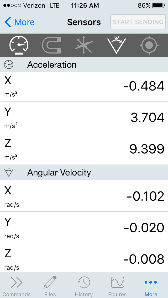
Modern mobile devices (smartphones, tablets, etc.) are equipped with various sensors that are used in general operation of the devices and in applications such as navigation and gaming. Two very common sensors are the three-axis accelerometer and the three-axis rate gyroscope that comprise a device’s inertial measurement unit (IMU). These sensors provide measurements of specific force (i.e., the difference between the absolute acceleration of the IMU and gravitational acceleration) and angular velocity with respect to their mutually perpendicular axes that corotate with the mobile device. With data analysis in mind, a convenient method for accessing these sensors’ signals is to use MATLAB Mobile. Simply put, using the MATLAB Mobile app on an iOS or Android mobile device, we can set up the device to communicate with MATLAB running on, say, a laptop, which allows us to transmit and record real-time measurements from the device’s three-axis accelerometer and rate gyroscope. In our case, we collected specific force and angular velocity data for an iPhone SE that was tossed roughly vertically in such a way to make it tumble. Figure 1 contains a screenshot of the phone in the MATLAB Mobile app with instantaneous values of the accelerometer and rate gyroscope signals displayed. The data were captured at the highest allowable sampling rate of 100 Hz. For the details of setting up MATLAB Mobile for real-time data collection, we refer the interested reader to MathWorks’ documentation here.

**Figure 1.** Screenshot of the MATLAB Mobile app on an iPhone SE displaying real-time readings from the phone’s three-axis accelerometer and rate gyroscope.

Equations of motion

Referring to Figure 2, the iPhone’s three-axis accelerometer and rate gyroscope provide specific force measurements $f_{i} = f_{i}(t)$ $(i = 1, \, 2, \, 3)$ and angular velocity signals $\omega_{i} = \omega_{i}(t)$ , respectively, with respect to phone-fixed axes aligned with the corotational basis $\{ \mathbf{e}_{1}, \, \mathbf{e}_{2}, \, \mathbf{e}_{3} \}$ . The illustrated corotational axes are consistent with those specified in MathWorks’ MATLAB Mobile documentation. We locate the position of the phone’s IMU relative to a fixed origin using a set of Cartesian coordinates, $x_{i} = \mathbf{x} \cdot \mathbf{E}_{i}$ , where $\{ \mathbf{E}_{1}, \, \mathbf{E}_{2}, \, \mathbf{E}_{3} \}$ is the space-fixed basis. The bases $\{ \mathbf{E}_{1}, \, \mathbf{E}_{2}, \, \mathbf{E}_{3} \}$ and $\{ \mathbf{e}_{1}, \, \mathbf{e}_{2}, \, \mathbf{e}_{3} \}$ are related by a rotation, which we choose to parameterize using a 3-2-1 set of Euler angles: $\psi$ , $\theta$ , and $\phi$ . Consequently, the forthcoming procedure for reconstructing the phone’s motion from the collected kinematic data closely follows the developments in our previous discussion of strapdown inertial navigation.

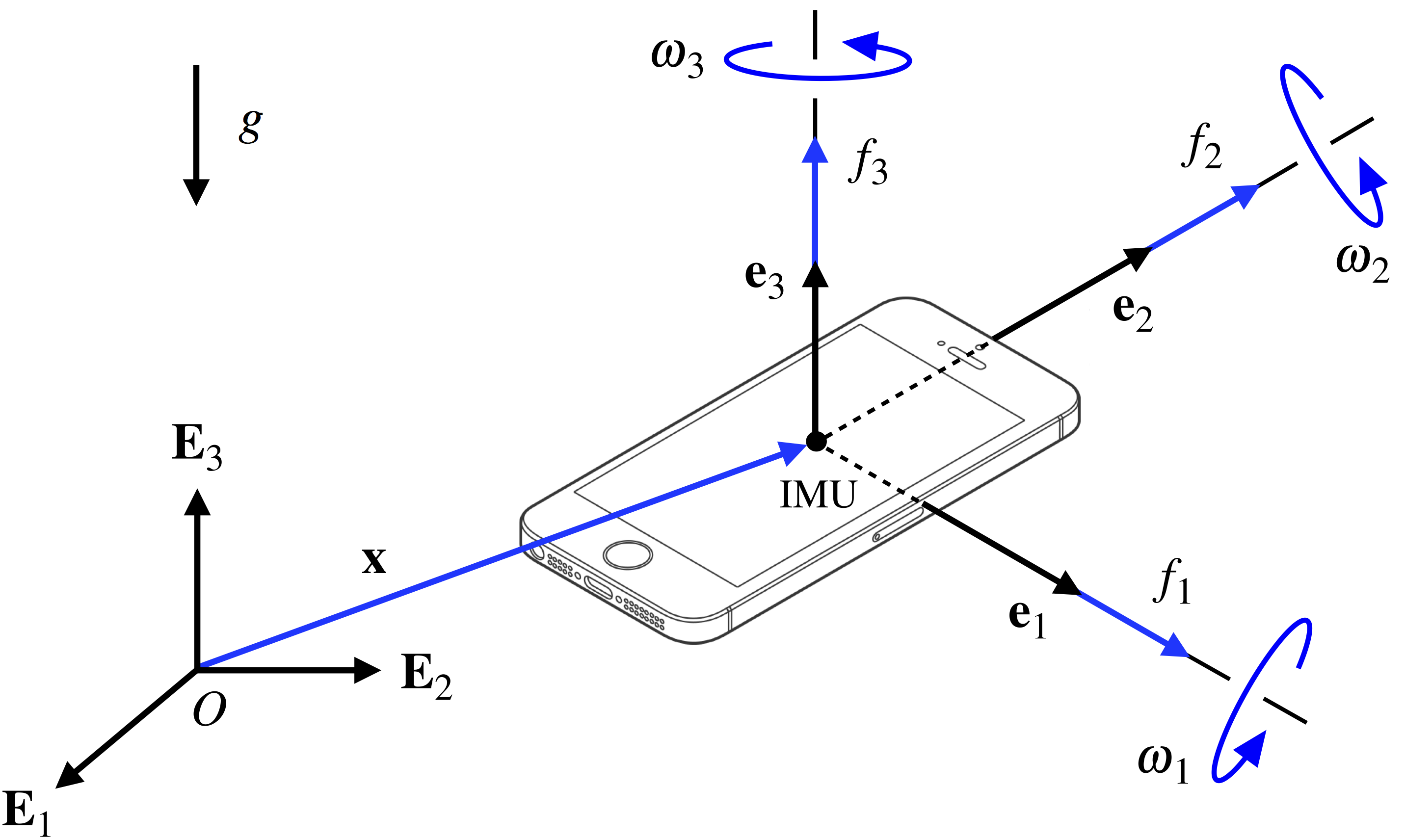
**Figure 2.** Schematic of an iPhone SE illustrating the alignment of the corotational axes and basis $\{ \mathbf{e}_{1}, \, \mathbf{e}_{2}, \, \mathbf{e}_{3} \}$ associated with the specific force and angular velocity measurements from the IMU’s three-axis accelerometer and rate gyroscope, respectively. The iPhone drawing was modified from an Apple Inc. image available here.

**Figure 2.** Schematic of an iPhone SE illustrating the alignment of the corotational axes and basis $\{ \mathbf{e}_{1}, \, \mathbf{e}_{2}, \, \mathbf{e}_{3} \}$ associated with the specific force and angular velocity measurements from the IMU’s three-axis accelerometer and rate gyroscope, respectively. The iPhone drawing was modified from an Apple Inc. image available here.

We first compute how the phone’s orientation varies when tossed in the air by integrating the following system of differential equations that relate the corotational angular velocity measurements $\omega_{i}(t)$ to the rates of change of the 3-2-1 Euler angles $\psi$ , $\theta$ , and $\phi$ :

(1) $\begin{equation*} \left[ \begin{array}{c} \dot{\psi} \\ \dot{\theta} \\ \dot{\phi} \end{array} \right] = \left[ \begin{array}{c c c } 0 & \sin(\phi) \sec(\theta) & \cos(\phi) \sec(\theta) \\ 0 & \cos(\phi) & - \sin(\phi) \\ 1 & \sin(\phi) \tan(\theta) & \cos(\phi) \tan(\theta) \end{array} \right] \left[\begin{array}{c} \omega_{1}(t) \\ \omega_{2}(t) \\ \omega_{3}(t) \end{array} \right] . \end{equation*}$

Notice that system (1) is conveniently already in the first-order form $\dot{\mathsf{y}} = \mathsf{f}(t, \, \mathsf{y})$ suitable for numerical integration in MATLAB, where the state vector $\mathsf{y} = \left [ \psi, \ \theta, \ \phi \right ]^{T}$ . Next, using the results for $\psi(t)$ , $\theta(t)$ , and $\phi(t)$ from integrating (1), we transform the corotational specific force measurements $f_{i}(t)$ into space-fixed components, $F_{i}(t)$ . For a 3-2-1 set of Euler angles, this is accomplished as follows:

(2) $\begin{equation*} \left[ \begin{array}{c} F_{1}(t) \\ F_{2}(t) \\ F_{3}(t) \end{array}\right] = \left[ \begin{array}{c c c } \cos(\psi) & -\sin(\psi) & 0 \\ \sin(\psi) & \cos(\psi) & 0 \\ 0 & 0 & 1 \end{array} \right] \left[ \begin{array}{c c c } \cos(\theta) & 0 & \sin(\theta) \\ 0 & 1 & 0 \\ - \sin(\theta) & 0 & \cos(\theta) \end{array} \right] \left[ \begin{array}{c c c } 1 & 0 & 0 \\ 0 & \cos(\phi) & -\sin(\phi) \\ 0 & \sin(\phi) & \cos(\phi) \end{array} \right] \left[ \begin{array}{c} f_{1}(t) \\ f_{2}(t) \\ f_{3}(t) \end{array} \right] . \hspace{1in} \scalebox{0.001}{\textrm{\textcolor{white}{.}}} \end{equation*}$

We then obtain the IMU’s absolute vertical acceleration $\ddot{x}_{3}(t)$ by, in principle, subtracting away gravitational acceleration $g$ from the vertical specific force component $F_{3}(t)$ . In practice, because of uncertainty in $g$ due to sensor noise, we extract $\ddot{x}_{3}(t)$ by removing the mean of $F_{3}(t)$ from the signal:

(3) $\begin{equation*} \ddot{x}_{3}(t) = F_{3}(t) - \overline{F}_{\!\!3}, \end{equation*}$

where the superposed bar denotes the mean value. The lateral specific force components $F_{1}(t)$ and $F_{2}(t)$ coincide with the IMU’s absolute lateral accelerations $\ddot{x}_{1}(t)$ and $\ddot{x}_{2}(t)$ , respectively. However, because of sensor bias, $F_{1}(t)$ and $F_{2}(t)$ might not have zero mean as expected; that is, the signals should closely fluctuate about zero when the phone is stationary, but these fluctuations might instead be offset from zero. Therefore, we take the accelerations $\ddot{x}_{j}(t)$ $(j = 1, \, 2)$ to be the specific force signals $F_{j}(t)$ corrected for sensor bias by subtracting away their respective mean values:

(4) $\begin{equation*} \ddot{x}_{j}(t) = F_{j}(t) - \overline{F}_{\!\!j}. \end{equation*}$

This process of removing the mean is often referred to as zero-centering. Lastly, we perform two successive integrations of each component of absolute acceleration, $\ddot{x}_{i}(t)$ , to determine the displacement components of the phone’s IMU during the toss:

(5) $\begin{equation*} x_{i}(t) = x_{i}(t_{0}) \, + \int_{t_{0}}^{t} \left ( \dot{x}_{i}(t_{0}) \, + \int_{t_{0}}^{\tau} \ddot{x}_{i}(u) \, \textrm{d} u \right ) \textrm{d} \tau . \end{equation*}$

Simulation and animation

The phone is initially in an unrotated state, and we take the starting location of its IMU to be the origin: $\psi(t_{0}) = \theta(t_{0}) = \phi(t_{0}) = 0$ and $x_{i}(t_{0}) = 0$ . In addition, the phone is initially at rest before being tossed, and so $\dot{x}_{i}(t_{0}) = 0$ . The specific force and angular velocity measurements were cropped so that processing of the data for motion reconstruction began just before the toss is initiated; removing the unnecessary measurements leading up to the toss helped alleviate the effect of integration drift. After obtaining the estimates of the phone’s orientation and displacement, we truncated the results to focus on the relevant motion between when the phone is tossed and when it is caught on the way down. The reconstructed motion of the tossed phone is animated in Figure 3.

Figure 3. Animation of the tossed iPhone’s tumbling motion reconstructed from onboard specific force and angular velocity measurements captured by the phone’s IMU. The animation was recorded at 3x slower speed.

Overall, the estimated behavior in Figure 3 is quite realistic, especially the tumbling itself, but we observe that the phone’s lateral displacement suffers from some integration drift, particularly in the $x_{2}$ coordinate. However, this result is far better than the motion we would obtain if we did not zero-center the absolute lateral acceleration components $\ddot{x}_{1}(t)$ and $\ddot{x}_{2}(t)$ as we did in (4). For our data, the absolute lateral specific force signal $F_{1}(t)$ has a small offset of about −0.075 m/s² that exacerbates the problem of integration drift, but not by much. On the other hand, the bias in $F_{2}(t)$ is over 20 times larger in magnitude at approximately 1.56 m/s², which, if not corrected for, results in a lateral motion $x_{2}(t)$ that is so exaggerated and unrealistic that it is comical. Figure 4 demonstrates how the reconstructed motion is negatively affected when $\ddot{x}_{1}(t)$ and $\ddot{x}_{2}(t)$ are not zero-centered.

Figure 4. Animation of the tossed iPhone’s reconstructed tumbling motion when the absolute lateral acceleration components $\ddot{x}_{1}(t)$ and $\ddot{x}_{2}(t)$ are not zero-centered. The effect on the displacement $x_{1}(t)$ is slight, but $x_{2}(t)$ experiences excessive and unrealistic drift. The animation was recorded at 3x slower speed.

Downloads

The animations in Figures 3 and 4 were generated using the MATLAB code provided below. Many thanks to Prithvi Akella for his assistance in developing this code and collecting data.

Main script:	Solve the equations of motion for the iPhone’s motion
Supporting files:	Define the rotational equations of motion Animate the iPhone’s motion Accelerometer and rate gyroscope data iPhone front and back images

** Unzip the downloaded file to extract the contents in .mat format.