Strapdown inertial navigation

The second problem in tracking and navigation is concerned with estimating the location and orientation of a body for which we have onboard kinematic measurements. Inertial measurement units (IMUs) consist of a set of three accelerometers placed to make acceleration-related measurements and a set of three rate gyroscopes that sense angular velocities in three mutually perpendicular directions. Here, we discuss the manner in which these signals can be used to determine the location and orientation of the body to which the IMU is rigidly attached. This process is known as strapdown inertial navigation [1, 2].

Contents

Signals from an inertial measurement unit

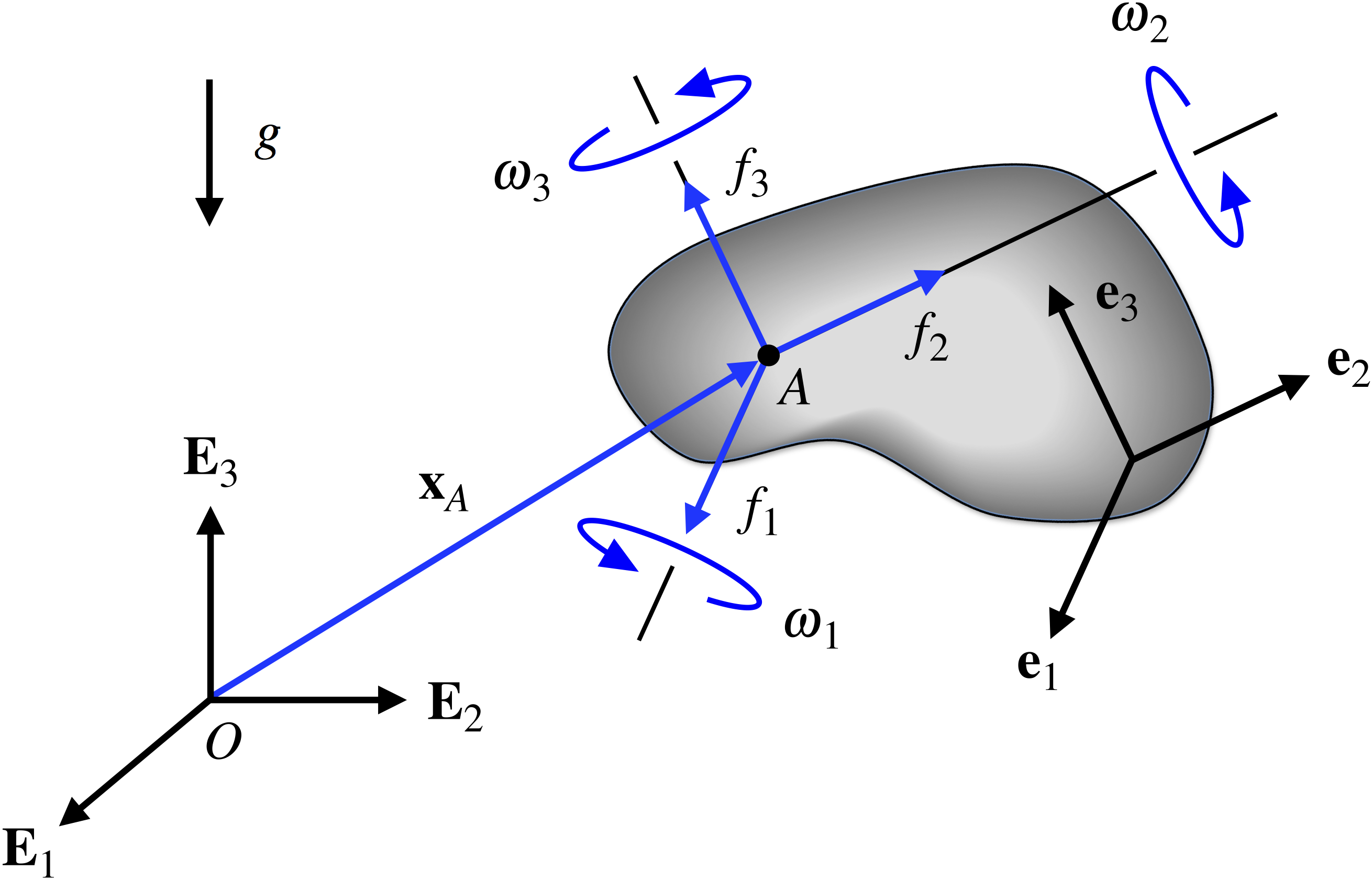
Referring to Figure 1, suppose the motion of a rigid body is characterized by a rotation tensor $\mathbf{Q}$ and the position vector $\mathbf{x}_A$ of a point $A$ on the body where an IMU is attached. The point $A$ is sometimes called a landmark. The rotation tensor $\mathbf{Q}$ relates the fixed, right-handed Cartesian basis $\{ \mathbf{E}_1, \, \mathbf{E}_2, \, \mathbf{E}_3 \}$ to the body’s corotational basis $\{ \mathbf{e}_1, \, \mathbf{e}_2, \, \mathbf{e}_3 \}$ , which we assume is aligned with the accelerometers’ and rate gyroscopes’ axes.

**Figure 1.** Schematic of a rigid body with landmark $A$ at which an IMU is attached. The axes associated with the IMU’s accelerometers and rate gyroscopes are aligned with the corotational basis $\{ \mathbf{e}_1, \, \mathbf{e}_2, \, \mathbf{e}_3 \}$ .

The IMU’s rate gyroscopes measure the components of the rigid body’s absolute angular velocity $\bomega$ in the corotational basis. That is, the rate gyroscopes provide the signals

(1) $\begin{equation*} \omega_i(t) = \bomega \cdot \mathbf{e}_i \quad (i = 1, \, 2, \, 3) . \end{equation*}$

The IMU’s accelerometers sense the corotational components of the so-called specific force $\mathbf{f}$ exerted at the landmark $A$ . Specific force is simply the difference between the absolute acceleration of $A$ , $\ddot{\mathbf{x}}_A$ , and gravitational acceleration, and thus the output of the accelerometers, $f_i(t)$ , can be identified with the measurements

(2) $\begin{equation*} f_i(t) = \mathbf{f} \cdot \mathbf{e}_i = \left ( \ddot{\mathbf{x}}_A - \mathbf{g} \right ) \cdot \mathbf{e}_i . \end{equation*}$

The navigation equations

Suppose a 3-2-1 set of Euler angles is used to parameterize $\mathbf{Q}$ . In vehicle dynamics, the Euler angles $\psi$ , $\theta$ , and $\phi$ are identified as the yaw, pitch, and roll angles, respectively. For this set of Euler angles, provided rate gyroscope data $\omega_i(t)$ , the orientation of the rigid body is determined by integrating the following set of differential equations:

(3) $\begin{equation*} \left[ \begin{array}{c} \dot{\psi} \\ \dot{\theta} \\ \dot{\phi} \end{array} \right] = \left[ \begin{array}{c c c } 0 & \sin(\phi) \sec(\theta) & \cos(\phi) \sec(\theta) \\ 0 & \cos(\phi) & - \sin(\phi) \\ 1 & \sin(\phi) \tan(\theta) & \cos(\phi) \tan(\theta) \end{array} \right] \left[\begin{array}{c} \omega_1 \\ \omega_2 \\ \omega_3 \end{array} \right] , \end{equation*}$

for which we must specify the body’s initial orientation: $\psi (t_0 )$ , $\theta (t_0 )$ , and $\phi (t_0 )$ . You may have noticed that these equations relating the rates of change of the Euler angles and $\omega_i$ can be obtained using the dual Euler basis vectors: $\dot{\psi} = \bomega \cdot \mathbf{g}^1$ , $\dot{\theta} = \bomega \cdot \mathbf{g}^2$ , and $\dot{\phi} = \bomega \cdot \mathbf{g}^3$ . Further, these equations are singular when $\theta = \pm \frac{\pi}{2}$ rad.

To solve for how the position vector $\mathbf{x}_A$ of the landmark $A$ varies over time, we first transform the corotational components of specific force, $f_i(t)$ , measured by the accelerometers into the fixed Cartesian frame and then correct for gravitational acceleration to obtain the fixed Cartesian components of the absolute acceleration of $A$ , $\ddot{x}_{A_i}(t) = \ddot{\mathbf{x}}_A \cdot \mathbf{E}_i$ . If we consider motion near the earth’s surface, then the gravitational acceleration vector $\mathbf{g} \approx -g \mathbf{E}_3$ . Consequently,

(4) $\begin{equation*} \left[ \begin{array}{c} \ddot{x}_{A_1} \! \\ \ddot{x}_{A_2} \! \\ \ddot{x}_{A_3} \! \end{array}\right] = \left[ \begin{array}{c c c } \cos(\psi) & -\sin(\psi) & 0 \\ \sin(\psi) & \cos(\psi) & 0 \\ 0 & 0 & 1 \end{array} \right] \left[ \begin{array}{c c c } \cos(\theta) & 0 & \sin(\theta) \\ 0 & 1 & 0 \\ - \sin(\theta) & 0 & \cos(\theta) \end{array} \right] \left[ \begin{array}{c c c } 1 & 0 & 0 \\ 0 & \cos(\phi) & -\sin(\phi) \\ 0 & \sin(\phi) & \cos(\phi) \end{array} \right] \left[ \begin{array}{c} f_{1} \\ f_{2} \\ f_{3} \end{array} \right] + \left[ \begin{array}{c} 0 \\ 0 \\ -g \end{array} \right] . \hspace{1in} \scalebox{0.001}{\textrm{\textcolor{white}{.}}} \end{equation*}$

We then twice integrate the system of differential equations (4), with initial position $x_{A_i} (t_0 )$ and velocity $\dot{x}_{A_i} (t_0 )$ , to obtain the trajectory of $A$ . Expressions (3) and (4) are often referred to as the navigation equations. The process we described here for computing the displacement of point $A$ and the body’s orientation over time using the IMU accelerometer and gyroscope data is summarized diagrammatically in Figure 2.

**Figure 2.** Diagrammatic representation of the process for calculating the displacement of a tracked point on a rigid body and the body’s orientation over time from IMU accelerometer and rate gyroscope data.

Integration drift and navigation error

In principle, numerically integrating (3) and (4) is not difficult. However, because of the inherent errors in numerical integration, the predicted orientation and location of the IMU will not correspond to the actual attitude and location. In fact, the discrepancies between the computed and actual orientation and position will increase over time. This phenomenon is known as integration drift, and it is unavoidable in inertial navigation systems. Unfortunately, the presence of noise in the IMU data, $f_i(t)$ and $\omega_i(t)$ , further amplifies errors in the estimated orientation and location. The use of accurate, but very expensive, IMUs slows the effect of integration drift and alleviates the issue of sensor noise, but a more effective strategy for managing integration drift would involve using other navigation aides such as GPS signals, magnetometers, and speedometer signals to supplement the IMU data and periodically correct the computed attitude and position.

To illustrate the effect of integration drift, consider an IMU attached to the center $A$ of a vehicle that travels at a constant speed in a circle of radius $R_0$ in the horizontal plane, as shown in Figure 3, where $\psi$ denotes the vehicle’s yaw angle.

**Figure 3.** Top-view schematic of a vehicle illustrating the alignment of the corotational basis vectors $\mathbf{e}_1$ and $\mathbf{e}_2$ as the vehicle travels in a circle.

If the initial conditions for the vehicle are such that $\mathbf{x}_A(0) = R_0 \mathbf{E}_1$ , $\dot{\mathbf{x}}_A(0) = \omega_0 R_0 \mathbf{E}_2$ , and $\psi(0) = 0$ , then the exact solutions for the position of $A$ and the vehicle’s orientation are given by

(5) $\begin{eqnarray*} && \mathbf{x}_A(t) = R_0 \left ( \cos(\omega_0 t) \mathbf{E}_1 + \sin(\omega_0 t) \mathbf{E}_2 \right ) , \\ \\ && \psi(t) = \omega_0 t . \end{eqnarray*}$

Because the vehicle’s motion is confined to the horizontal plane, the navigation equations (3) and (4) reduce to

(6) $\begin{eqnarray*} && \dot \psi = \omega_3 , \\ \\ && \left[ \begin{array}{c c c} \ddot{x}_{A_1} \! \\ \ddot{x}_{A_2} \! \end{array} \right] = \left[ \begin{array}{c c c } \cos(\psi) & -\sin(\psi) \\ \sin(\psi) & \cos(\psi) \end{array} \right] \left[ \begin{array}{c c c} f_{1} \\ f_{2} \end{array} \right] . \end{eqnarray*}$

Thus, (5) and (6) imply that the IMU must yield the following signals:

(7) $\begin{eqnarray*} && \omega_3(t) = \omega_0 , \\ \\ && f_1(t) = - \omega_0^2 R_0 , \\ \\ && f_2(t) = 0 . \end{eqnarray*}$

Figure 4 depicts the IMU signals (7) for $R_0 = 5$ m and $\omega_0 = \pi$ rad/s.

**Figure 4.** Noise-free angular velocity and specific force signals from an IMU attached to the center of a vehicle traveling in a circle at a constant speed.

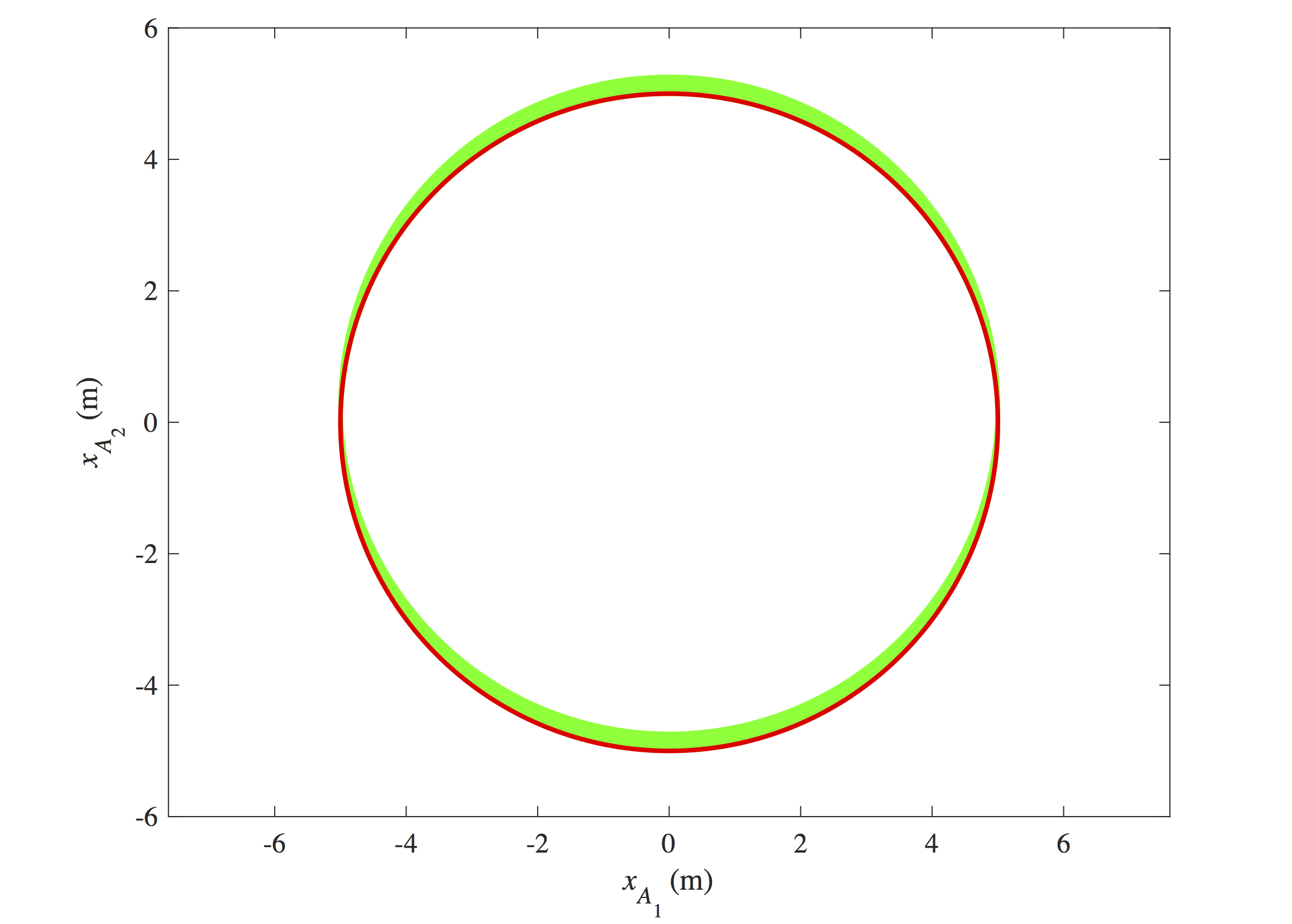
Now, suppose the IMU’s sampling rate is 100 Hz. If we solve the navigation equations (6) and integrate to compute the trajectory of the vehicle’s center $A$ , we find, as shown in Figure 5, that the estimated trajectory (drawn in green) noticeably deviates from the actual circular path (drawn in red) as time progresses. This integration drift is unavoidable, but its effect can be slowed if the IMU were to collect data at a higher sampling rate.

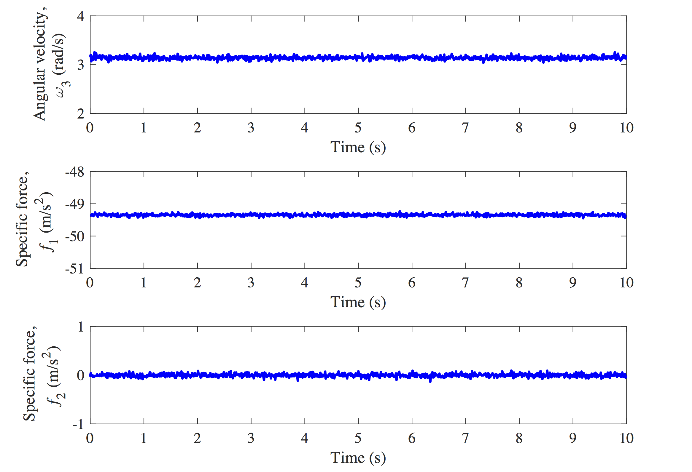
**Figure 5.** Illustration of integration drift for a vehicle traveling in a circle when the IMU data is free of noise. The computed trajectory of the vehicle’s center is shown in green, while the actual circular path is drawn in red.

Of course, the IMU data will be subject to noise, and therefore the angular velocity and specific force signals (7) are depicted more realistically in Figure 6.

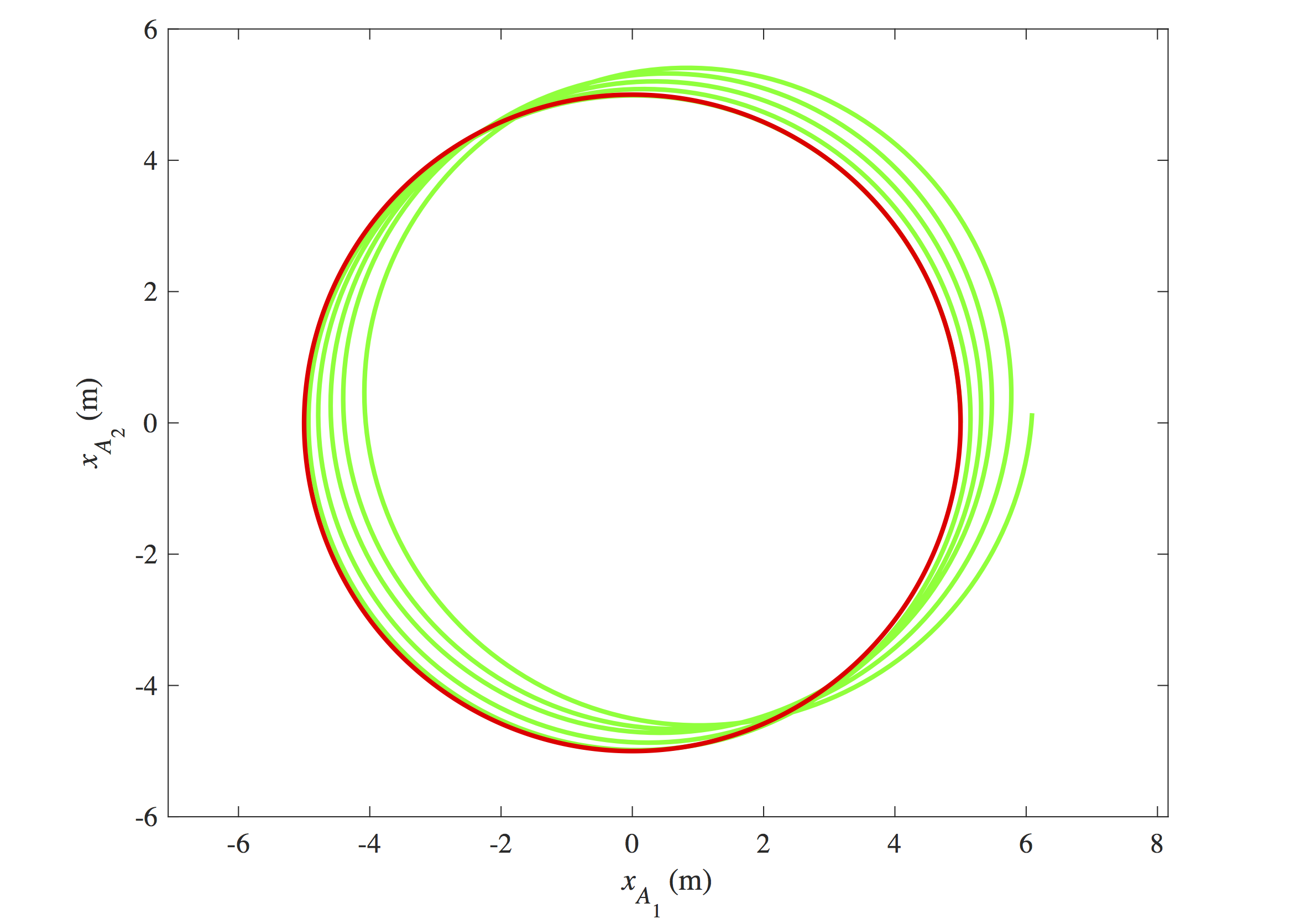
**Figure 6.** Noisy angular velocity and specific force signals from an IMU attached to the center of a vehicle traveling in a circle at a constant speed.

As expected, we see in Figure 7 that the presence of noise in the data exacerbates the effect of integration drift, quickly resulting in a significant discrepancy between the estimated trajectory of $A$ (draw in green) and the actual circular path (drawn in red).

**Figure 7.** Illustration of integration drift for a vehicle traveling in a circle when the IMU data is noisy. The computed trajectory of the vehicle’s center is shown in green, while the actual circular path is drawn in red.

Downloads

The MATLAB code used to create Figures 4–7 is available here. Please note that the noise added to the ideal IMU signals shown in Figure 4 is generated randomly, so executing this code on your machine will yield results that are similar, but not necessarily identical, to those depicted in Figures 6 and 7.

References

Britting, K. R., Inertial Navigation Systems Analysis, John Wiley & Sons, Inc., New York (1971). Reprinted by Artech House in 2010.
Titterton, D. H., and Weston, J. L., Strapdown Inertial Navigation Technology, 2nd ed., The Institution of Electrical Engineers, Stevenage, United Kingdom (2004).