A tumbling T-handle in space: the Dzhanibekov effect

The video in Figure 1 of a tumbling T-handle on the International Space Station is a wonderful illustration of the instability of rotation about an asymmetric object’s intermediate principal axis. This instability is also known as the Dzhanibekov effect after the Soviet cosmonaut Vladimir Dzhanibekov who discovered this effect on the MIR space station in 1985. The T-handle’s rotational motion is well approximated by considering the object to be rigid and modeling its rotational behavior via a balance of angular momentum.

Figure 1. A T-handle tumbling in space aboard the International Space Station.

Contents

Equations of motion

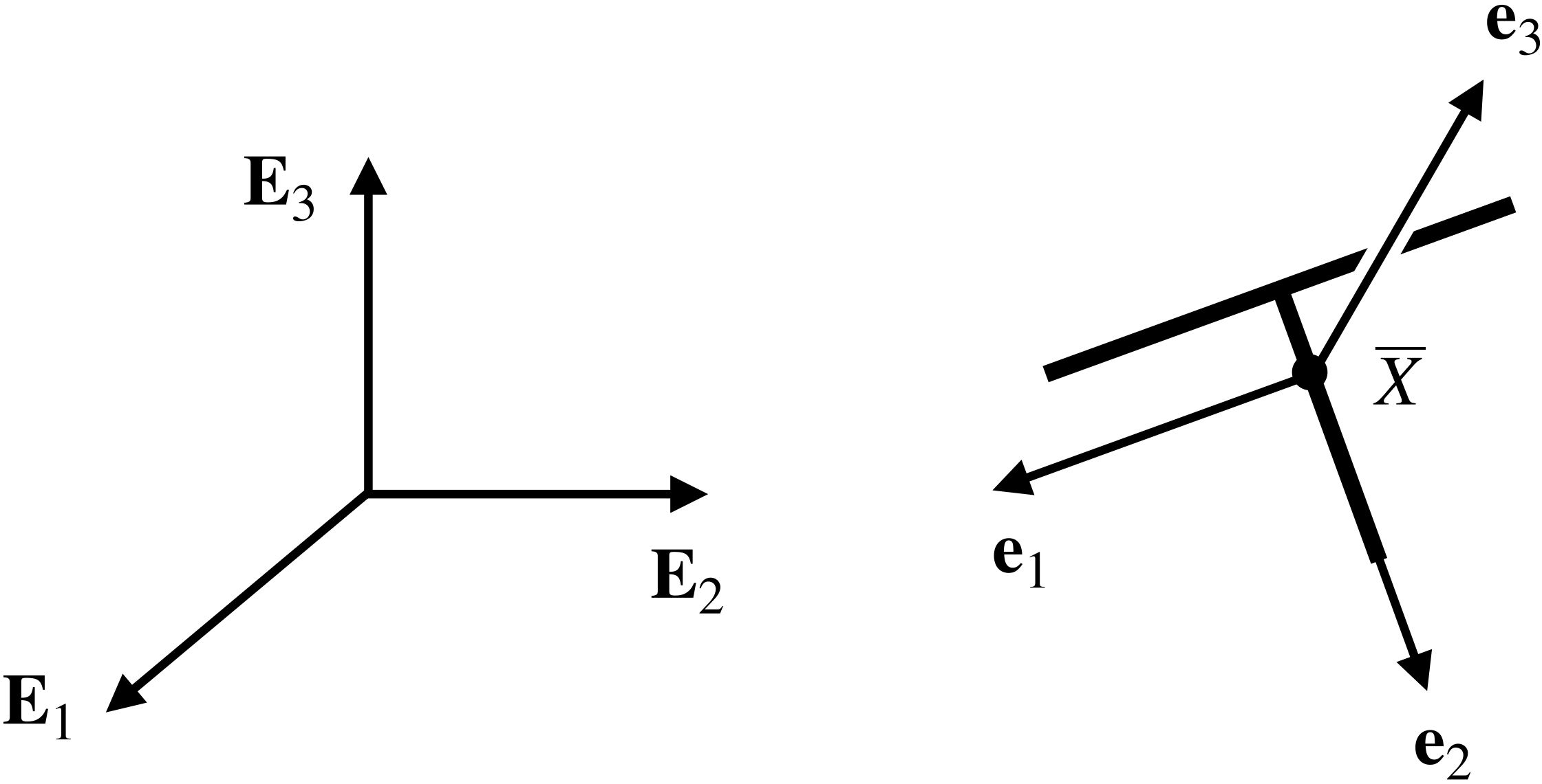
Suppose we parameterize the rotation of the T-handle by a 3-1-3 set of Euler angles: $\psi$ , $\theta$ , and $\phi$ . As illustrated in Figure 2, this sequence of rotations relates the space-fixed basis $\{ \mathbf{E}_{1}, \, \mathbf{E}_{2}, \, \mathbf{E}_{3} \}$ to the corotational basis $\{ \mathbf{e}_{1}, \, \mathbf{e}_{2}, \, \mathbf{e}_{3} \}$ associated with the T-handle’s principal axes, with the intermediate axis aligned with the object’s longitudinal axis.

**Figure 2.** Schematic of a T-handle illustrating the alignment of the corotational basis $\{ \mathbf{e}_{1}, \, \mathbf{e}_{2}, \, \mathbf{e}_{3} \}$ .

**Figure 2.** Schematic of a T-handle illustrating the alignment of the corotational basis $\{ \mathbf{e}_{1}, \, \mathbf{e}_{2}, \, \mathbf{e}_{3} \}$ .

The angular momentum of the T-handle about its mass center $\overline{X}$ is given by $\mathbf{H} = \sum_{i \, \, = \, 1}^{3} \lambda_{i} \omega_{i} \mathbf{e}_{i}$ , where $\lambda_{i}$ are the principal moments of inertia (which are distinct for an asymmetric body) and $\omega_{i}$ are the corotational components of angular velocity: $\omega_{i} = \bomega \cdot \mathbf{e}_{i}$ . Neglecting the small resultant moment acting on the T-handle due to the central force field while orbiting the earth, a balance of angular momentum with respect to the mass center yields $\dot{\mathbf{H}} = \mathbf{0}$ , resulting in the equations of motion

(1) $\begin{eqnarray*} && \lambda_{1} \dot \omega_{1} = - (\lambda_{3} - \lambda_{2}) \omega_{2} \omega_{3} , \\ \\ && \lambda_{2} \dot \omega_{2} = - (\lambda_{1} - \lambda_{3}) \omega_{1} \omega_{3} , \\ \\ && \lambda_{3} \dot \omega_{3} = - (\lambda_{2} - \lambda_{1}) \omega_{1} \omega_{2} . \end{eqnarray*}$

For a 3-1-3 set of Euler angles, $\omega_{i}$ are related to the Euler angles $\psi$ , $\theta$ , and $\phi$ and their rates of change as follows:

(2) $\begin{eqnarray*} && \omega_{1} = \dot \psi \sin(\theta) \sin(\phi) + \dot \theta \cos(\phi) , \\ \\ && \omega_{2} = \dot \psi \sin(\theta) \cos(\phi) - \dot \theta \sin(\phi) , \\ \\ && \omega_{3} = \dot \psi \cos(\theta) + \dot \phi . \end{eqnarray*}$

Sets (1) and (2) constitute a system of first-order differential equations that solve for the T-handle’s orientation over time. These equations may be conveniently expressed in the form $\mathsf{M}(t, \, \mathsf{y}) \dot{\mathsf{y}} = \mathsf{f}(t, \, \mathsf{y})$ for numerical integration in MATLAB, where we take the state vector $\mathsf{y} = \left [ \omega_{1}, \ \omega_{2}, \ \omega_{3}, \ \psi, \ \theta, \ \phi \right ]^{T}$ :

(3) $\begin{eqnarray*} && \mathsf{M}(t, \, \mathsf{y}) = \left[ \begin{array}{c c c c c c} \lambda_{1} & 0 & 0 & 0 & 0 & 0 \\ 0 & \lambda_{2} & 0 & 0 & 0 & 0 \\ 0 & 0 & \lambda_{3} & 0 & 0 & 0 \\ 0 & 0 & 0 & \sin(\theta) \sin(\phi) & \cos(\phi) & 0 \\ 0 & 0 & 0 & \sin(\theta) \cos(\phi) & -\sin(\phi) & 0 \\ 0 & 0 & 0 & \cos(\theta) & 0 & 1 \end{array} \right], \hspace{1in} \scalebox{0.001}{\textrm{\textcolor{white}{.}}} \\ \\ \\ && \mathsf{f}(t, \, \mathsf{y}) = \left[ \begin{array}{c} - (\lambda_{3} - \lambda_{2}) \omega_{2} \omega_{3} \\ - (\lambda_{1} - \lambda_{3}) \omega_{1} \omega_{3} \\ - (\lambda_{2} - \lambda_{1}) \omega_{1} \omega_{2} \\ \omega_{1} \\ \omega_{2} \\ \omega_{3} \\ \end{array} \right]. \end{eqnarray*}$

Simulation and animation

To demonstrate instability of rotation about the intermediate principal axis, suppose the T-handle is initially spinning about this axis at a rate $\Omega$ with small perturbations $\altepsilon << \Omega$ in the initial angular velocity about the other two principal axes: $\bomega(t_0) = \altepsilon \mathbf{e}_{1} + \Omega \mathbf{e}_{2} + \altepsilon \mathbf{e}_{3}$ . For convenience, let the T-handle’s initial orientation be defined as $\psi(t_0) = 0$ , $\theta(t_0) = \frac{\pi}{2}$ rad (to avoid the singularity in the 3-1-3 set of Euler angles), and $\phi(t_0) = 0$ . The resulting motion of the T-handle, which is very similar to the observed behavior in Figure 1, is animated in Figure 3 for a particular choice of physical and simulation parameters. It can also be shown that the simulated motion conserves both energy and angular momentum: the energy $E = T_{\textrm{rot}} = \frac{1}{2} \sum_{i \, \, = \, 1}^{3} \lambda_{i} \omega_{i}^2 = \textrm{constant}$ , and $\Arrowvert \mathbf{H} \Arrowvert = \textrm{constant}$ .

Figure 3. Animation of the simulated tumbling behavior of a T-handle in space demonstrating the instability of rotation about the intermediate principal axis.

Downloads

The animation in Figure 3 was generated using the following MATLAB code:

Main script:	Solve the T-handle’s equations of motion
Supporting files:	Derive the T-handle’s equations of motion ** Animate the T-handle’s motion

** Run this code first to obtain the symbolic equations of motion called by the main script. (The Symbolic Math Toolbox is required.) This code needs to be run only once, before the first use of the main script.