A geodesic is a curve of shortest distance between two points on a manifold (surface). Classic examples include the geodesic between two points in a Euclidean space is a straight line and the geodesic between two points on a sphere is a great circle. Dating to Jacobi in the 1800s, it is known that for two points on a manifold  , a necessary condition for a geodesic between two points can be found by imagining a particle moving on (see, e.g., Lanczos [1]). The necessary condition is identical to the motion of the particle satisfying Lagrange’s equations of motion for the particle. That is, the path
  of the particle is a geodesic for pairs of points that passes through.
With respect to the simplest possible metric (measure of distance) for the group of rotations  , geodesics of are characterized by constant angular velocity motions of rigid bodies and, if quaternions are used to parameterize the rotation, as great circles on a three-sphere (cf. Figure 1). As discussed below, the former interpretation is employed used in optometry to characterize saccadic motions of the eye (see [2, 3, 4, 5, 6, 7, 8, 9, 10]) and the latter is the basis for the SLERP algorithm interpolation of rotations in computer graphics (see Shoemake [11]). The simplicity of these two disparate interpretations belies the complexity of the corresponding rotations. By using a quaternion representation for a rotation, a simple proof of the equivalence of the aforementioned characterizations and a straightforward method to establish features of the corresponding rotations are discussed. Our discussion is based on the recent papers by Novelia and O’Reilly [12, 13] and O’Reilly and Payen [14].
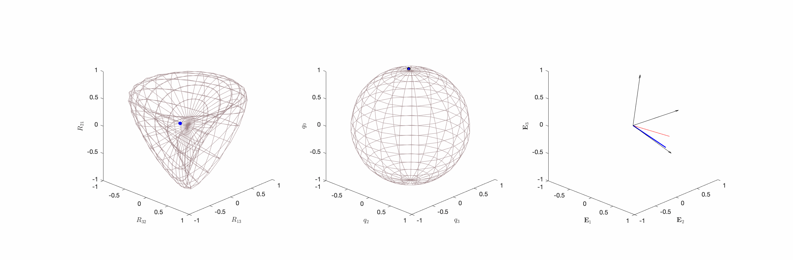
Figure 1. Three distinct representations of a class of constant angular velocity motion. From left to right, a representation using the components of
 and Steiner’s Roman Surface, a representation using a unit quaternion on a two-sphere, and a representation using the corotational basis vectors
  of a rigid body motion. This figure is adopted from Novelia and O’Reilly [13].
The choice of the simplest metric is equivalent to examining the moment-free rotational motions of a spherically symmetric rigid body. For such a rigid body, the moment of inertia tensor  is simply a scalar multiple of the identity and, using a balance of angular momentum,
  , we can conclude that the angular velocity vector
  is constant for all moment-free motions. Thus, if you throw a tennis ball into the air, and ignore drag, then it will rotate with a constant angular velocity. The rotation tensor
  of the ball describes a geodesic on with respect to the simplest metric. There are several methods to visualize the rotation: components of a quaternion on a three-sphere and an immersion using Steiner’s Roman surface. The immersion was first described by Apery [15] and can (surprisingly) be related to the components of the rotation tensors
  .
.
By changing the metric, the geodesics change. To observe this phenomenon, we again exploit the analogy with moment-free motion of a rigid body and consider axisymmetric and asymmetric rigid bodies. We again find that a subset of the geodesics correspond to motions with constant angular velocities, but also observe that more complex rotational motions of the rigid body can also serve as geodesics of .
Contents
The Euler-Rodrigues and quaternion parameterizations
The use of four Euler-Rodrigues symmetric (or Euler symmetric) parameters to parameterize a rotation dates to Euler [16] in 1771 and Rodrigues [17] in 1840 [18, 19, 20]. We denote these parameters by the pair  , where
  is a scalar and
  is a vector. In 1843, Hamilton [21] made his discovery of quaternion multiplication, and shortly afterwards Cayley [22] published results showing how quaternions could be used to parameterize a rotation. The historical development of these parameterizations features some of the greatest mathematicians of the 18th and 19th centuries. These individuals include Euler, Gauss [23], and Cayley, among others. The topic also provides a fascinating introduction to this period. For further details, we refer the reader to the works [18, 19, 20, 24, 25]. The use of quaternions to parameterize saccadic motions of the eye was successfully championed by Westheimer [10].
The Euler-Rodrigues symmetric parameters and satisfy the constraint
(1) 
Let the pair  , where
  is a scalar and
  is a vector, denote a unit quaternion, which has unit norm:
(2) 
Thus, a unit quaternion can be used to define a set of Euler-Rodrigues symmetric parameters, and vice versa:  and
and  . In the four-dimensional space parameterized by the components of a quaternion, the set of all unit quaternions defines a unit sphere referred to as the 3-sphere
  . The parameters and can be used to define a rotation about an axis
  through an angle
  using the identifications
(3) 
The resulting representation of the rotation tensor , which transforms the fixed basis  into the corotational basis
  , is given by
(4) 
 , one finds that the components are quadratic functions of the four parameters and :
(5) ![\begin{equation*}\mathsf{R} =\left[ \begin{array}{c c c}R_{11} & R_{12} & R_{13} \\R_{21} & R_{22} & R_{23} \\R_{31} & R_{32} & R_{33}\end{array} \right] = \left( 2 q^2_0 - 1 \right)\left[ \begin{array}{c c c}1 & 0 & 0 \\0 & 1 & 0 \\0 & 0 & 1\end{array} \right]+ 2\left[ \begin{array}{c c c}q^2_1 & q_1q_2 & q_1q_3 \\q_1q_2 & q^2_2 & q_2q_3 \\q_1q_3 & q_2q_3 & q^2_3\end{array} \right]+ 2q_0\left[ \begin{array}{ccc}0 & -q_3 & q_2 \\q_3 & 0 & -q_1 \\-q_2 & q_1 & 0\end{array}\right] . \hspace{1in} \scalebox{0.001}{\textrm{\textcolor{white}{.}}}\end{equation*}](https://rotations.berkeley.edu/wp-content/ql-cache/quicklatex.com-d3862e65f37cdb98327d32fd8c8c9a0b_l3.png "Rendered by QuickLaTeX.com")
Consequently, representation (4) is free of trigonometric functions and singularities, making it attractive from a numerical implementation standpoint. In addition, the fact that unit quaternions lie on the 3-sphere and can be used to represent rotations is exploited in computer graphics to interpolate animations (see Shoemake [11]). Examining (5) in closer detail,
(6) ![\begin{equation*}R_{ik} =\left[ \begin{array}{cccc}q_0 & q_1 & q_2 & q_3\end{array} \right]\mathsf{F}_{ik}\left[ \begin{array}{c}q_0 \\q_1 \\q_2 \\q_3\end{array}\right] ,\end{equation*}](https://rotations.berkeley.edu/wp-content/ql-cache/quicklatex.com-8fb51aa779d5cc75ded6dc5fb67ac112_l3.png "Rendered by QuickLaTeX.com")
where each of the nine 4  4 matrices
  are symmetric and proper-orthogonal. For example,
(7) ![\begin{eqnarray*}&& \mathsf{F}_{11} =\left[\begin{array}{cccc}1 & 0 & 0 & 0 \\0 & 1 & 0 & 0 \\0 & 0 & -1 & 0 \\0 & 0 & 0 & -1\end{array}\right],\\\\\\&& \mathsf{F}_{31} =\left[\begin{array}{cccc}0 & 0 & -1 & 0 \\0 & 0 & 0 & 1 \\-1 & 0 & 0 & 0 \\0 & 1 & 0 & 0\end{array}\right].\end{eqnarray*}](https://rotations.berkeley.edu/wp-content/ql-cache/quicklatex.com-7b0af7175bcee7e41ae5ccfff6120f3e_l3.png "Rendered by QuickLaTeX.com")
The matrices play a role in constructing stiffness matrices [26] and in establishing identities for the derivatives of the components of the matrix  [27].
[27].
In terms of and , the angular velocity vector  associated with has the well-known representation
(8) 
It is interesting to note that the time derivative of and its corotational rate  are simply related [26]:
(9) 
To verify this result, recall that  because
  . Computing
  and then using the identity
  confirms (9). With the help of (9), some lengthy but straightforward manipulations of (8) reveal that has the equivalent representation
(10) 
For completeness, we note that the angular velocity  , defined as the axial vector of
  , can be obtained from according to
(11) 
Using (10) and the identities , (9), and  for any vectors
  and
and  , it follows that has the representation
(12) 
As discussed in [28, 29], this representation is convenient to use when computing Lagrange’s equations of motion for rigid bodies. Lastly, taking the  components of representation (10) for leads to
(13) ![\begin{equation*}\left[ \begin{array}{c}\bomega_{\bf R}\cdot{\bf e}_1 \\\bomega_{\bf R}\cdot{\bf e}_2 \\\bomega_{\bf R}\cdot{\bf e}_3\end{array} \right] = \mathsf{C}\left[ \begin{array}{c}\dot{q}_0 \\\dot{q}_1 \\\dot{q}_2 \\\dot{q}_3\end{array} \right],\end{equation*}](https://rotations.berkeley.edu/wp-content/ql-cache/quicklatex.com-e87d0229a1b8e1a1493d0b87cf9b5826_l3.png "Rendered by QuickLaTeX.com")
where
(14) ![\begin{equation*}\mathsf{C} = 2\left[ \begin{array}{c c c c}-q_1 & q_0 & q_3 & -q_2 \\-q_2 & -q_3 & q_0 & q_1 \\-q_3 & q_2 & -q_1 & q_0\end{array} \right].\end{equation*}](https://rotations.berkeley.edu/wp-content/ql-cache/quicklatex.com-e7ad40f8b5e17c9f476c3b8e64bd4e6f_l3.png "Rendered by QuickLaTeX.com")
The  matrix
  has the generalized inverse
(15) 
That is,  , where
  is the 4 4 identity matrix. Thus, using
  , (13) can be rearranged to establish the following differential equations for the parameters and in terms of
  :
:
(16) ![\begin{equation*}\left[ \begin{array}{c}\dot{q}_0 \\\dot{q}_1 \\\dot{q}_2 \\\dot{q}_3\end{array} \right] = \frac{1}{2}\left[ \begin{array}{c c c}- q_1 & -q_2 & -q_3 \\q_0 & - q_3 & q_2 \\q_3 & q_0 & - q_1 \\-q_2 & q_1 & q_0\end{array} \right]\left[ \begin{array}{c}\omega_1 \\\omega_2 \\\omega_3\end{array} \right].\end{equation*}](https://rotations.berkeley.edu/wp-content/ql-cache/quicklatex.com-90a694e5654cd144370f0a4393c29d1a_l3.png "Rendered by QuickLaTeX.com")
Given measurements for  and the initial orientation
  and
and  of a body, these differential equations can be integrated to determine
  and
and  , and hence the body’s orientation
  .
.
Geodesics of SO(3): the simplest metric and the dynamics of a spherically symmetric body
The shortest distance between two points on a manifold depends on the measure of distance used on the manifold. The simplest metric for is based on the inner-product  where is the angular velocity vector associated with the rotation tensor
  . This choice of metric is equivalent to examining the moment-free motion of a spherically symmetric rigid body.
For a spherically symmetric rigid body of mass  and radius
  , the rotational kinetic energy of the rigid body is simply
  where is the angular velocity vector of the rigid body and is the associated rotation tensor. We can use this energy to define the kinematical line-element (or measure of distance)
  for :
for :
(17) 
Here,
(18) 
The geodesics with respect to are extremizers of  and, appealing to Jacobi’s theorem, we note that the rotational kinetic energy is conserved along the geodesics (see, e.g., Lanczos [1]). Conservation of also implies that the angular speed
  of the rotational motion that corresponds to the geodesic is constant.
If we use unit quaternions to parameterize , then a two-to-one covering of is obtained. That is, the pair of quaternions  and
and  , correspond to the same rotation. Unit quaternions can be considered as points on a 3-dimensional sphere that is embedded in a 4-dimensional Euclidean space. To explore the geodesics on , it is first convenient for illustrative purposes to consider geodesics of using the kinematical line-element . The necessary conditions for
  to correspond to a geodesic are established using a variational principle for geodesics on a configuration manifold. The resulting conditions are the Euler-Lagrange necessary condition:
(19) 
where  is a Lagrange multiplier associated with the Euler parameter constraint:
(20) 
Substituting for , (19) reduce to
(21) 
where  . These equations have the integral of motion and we denote the value of this integral of motion by
  . While our construction of (21) follows from a variational principle for geodesics on a configuration manifold, the corresponding equations of motion also follow from those for the rotational motion of a rigid body whose rotation is parameterized by Euler parameters.
With the help of (20), we follow [27, 29] and solve for :
(22) 
Hence, (19) reduce further to
(23) 
These equations imply that the quaternion components associated with a geodesic execute simple harmonic motions:
(24) 
where the frequency  is half the magnitude of :
(25) 
The factor of one half in the angular speed of  compared to
  can be attributed to the fact that the unit quaternions provide a two-to-one cover for . The initial conditions
  and
and  must satisfy the Euler parameter constraint
  and its differential counterpart
  .
.
While the angular speed associated with the geodesic motions is constant, this does not guarantee that is a constant. However, as
(26) 
and, from (21),  and
and  , we can conclude that is constant. Thus, geodesics on with respect to correspond to rotations with constant angular velocity vectors.
As discussed in [13], the path traced out by the unit quaternion given by (24) are arcs of great circles on the unit 3-sphere. That is, these are the motions used to interpolate rotation tensors in Shoemake’s SLERP algorithm [11].
The simplicity of the differential equations (23) governing , which were first presented in Novelia and O’Reilly [13], enables on to quickly conclude that and  lie on a plane by noting the constancy of
  :
:
(27) 
An alternative formulation of (23) is presented in O’Reilly and Payen [14]. Their resulting differential equations for the axis and angle  of a rotation corresponding to a constant angular velocity motion are integrable, equivalent to (23) but far more difficult to solve analytically:
(28) 
We invite the reader to compare (28) to the corresponding set of equations expressed using quaternions (23).
In the sequel, and without loss in generality, we often take advantage of the result that and lie on a plane by choosing  such that
  is normal to the aforementioned plane:
  . In this case, we can define the angle
  such that
(29) 
With the help of (24) it is straightforward to write down analytical expressions for  and
and  :
:
(30) 
The reader should observe that and  are not necessarily constant even though is. With reference to the ordinary differential equations (28),
  .
.
Geodesics of SO(3): the simplest metric and the immersion of the real projective plane
Allowing for the fact that we can choose  without loss in generality, the remaining coordinates to parameterize are
  ,
,  and
and  . We know that the geodesics of are circles on a two-sphere
  in
in  . The sphere, however, still retains the two-to-one covering property between a pair of antipodal points and a rotation
  :
:  and its antipodal point
  describe the same rotation . It is a well-known result in topology that the quotient space of obtained by identifying antipodal points is the real projective plane
  . Consequently, points in are isomorphic to when (cf. [13, 15, 28, 30]). Unfortunately, can be embedded in
  but not . See, for example, Section 7 of the textbook by Tu [31] for a good discussion on projective spaces. O’Reilly’s exposition on these matters in Section 6 of [28] is heavily influenced by the discussion of
  in Tu [31].
To proceed further, we immerse into a non-orientable surface in which is known as Steiner’s Roman surface  . The transformation required to perform the immersion is discussed in Apery’s seminal work [15]:
(31) 
However, from the representation (5) for the components of a rotation tensor , we find that
(32) 
Thus by projecting into , we arrive at the desired mapping
(33) 
We next recast the parametric equations for the two-dimensional manifold , known as Steiner’s Roman surface, in by representing the quaternion components as a function of azimuthal and zenith angles on :  (cf. (29)). The resulting expressions for the Cartesian coordinates of a point on are
(34) 
Although is a non-orientable surface in , all but three rotations can be identified with a single point on . The exceptions are the three rotations  ,
,  , and the identity
  . Each of these three rotations are mapped to the origin (also known as the triple point or pinch point of ). Because the rotations associated with the triple point are not unique, it is possible to have a closed trajectory starting from and ending at the triple point where the body does not return to its starting orientation.
Representative examples of geodesics of as they manifest as curves on are shown in Figures 2, 3, and 4. As discussed below, the representations of the geodesics of on are either straight lines or ellipses.
Representations of the geodesics of SO(3): the simplest metric and the rotation of a rigid body
The geodesic on when the simplest metric is employed correspond to rotational motions of a rigid body with a constant angular velocity vector:
(35) 
where  are constant. Consequently, the instantaneous axis
  is constant. However, these results in and of themselves do not provide the full picture of the behavior of the rotation . We now examine different manifestations of rotations with constant angular velocities. An important point to note here is that the rotation tensors and
  where
where  is constant have the same angular velocity vectors but may have distinct angles and axes of rotation. This is equivalent to the fact that two motions of a particle may have the same velocity vector but they can have distinct position vectors.
Substituting the expressions (24) for into (5) , the resulting rotation tensor and can be found. It is easier however to present some qualitative observations. First, we note that is constant for the geodesics and hence the projection of onto is constant. Because the magnitude of is 1, we can conclude that describes an arc of a circle during its motion. The circle in question is centered at a point along the instantaneous axis of rotation  .
.
Because of the definitions of quaternion components  , we immediately conclude from (24) that the period of is half that of the quaternion components while the period of is the same as those for the quaternion components. Thus,
  . To gain further insight, we appeal to the identity relating
  to :
to :
(36) 
This expression, along with (23) (i.e.,  ) can also be used to establish an expression for
  . It is easy to then show that
  . This result, which was first established in O’Reilly and Payen [14], implies that either is constant or it traces a great circle.
Choosing to be normal to (without loss of generality), we previously arrived at the analytical expressions (30) for and . Consequently, we appeal to [14] who found that rotations with constant angular velocity motions can be classified into three types:
- Type I Motions where the axis of rotation is parallel to and is a non-zero constant:
 and
and  (cf. Figure 2).
 - Type II Motions where
 and the axis of rotation is perpendicular to . That is,
  and
and  (cf. Figure 3).
 - Type III. Motions where
 but is neither normal to nor parallel to . That is,
  and
and  (cf. Figure 4).
Type I motions are prototypical constant angular velocity motions and, given the freedom to choose the reference basis  or, equivalently, , constant angular velocity motions can always be restricted to this type. For motions of this type
  at some instant
  and this guarantees that the constant will be parallel to the axis of rotation . Unfortunately, in many application areas, such as opthomology, the reference basis for is prescribed and Type II and Type III motions must be considered.
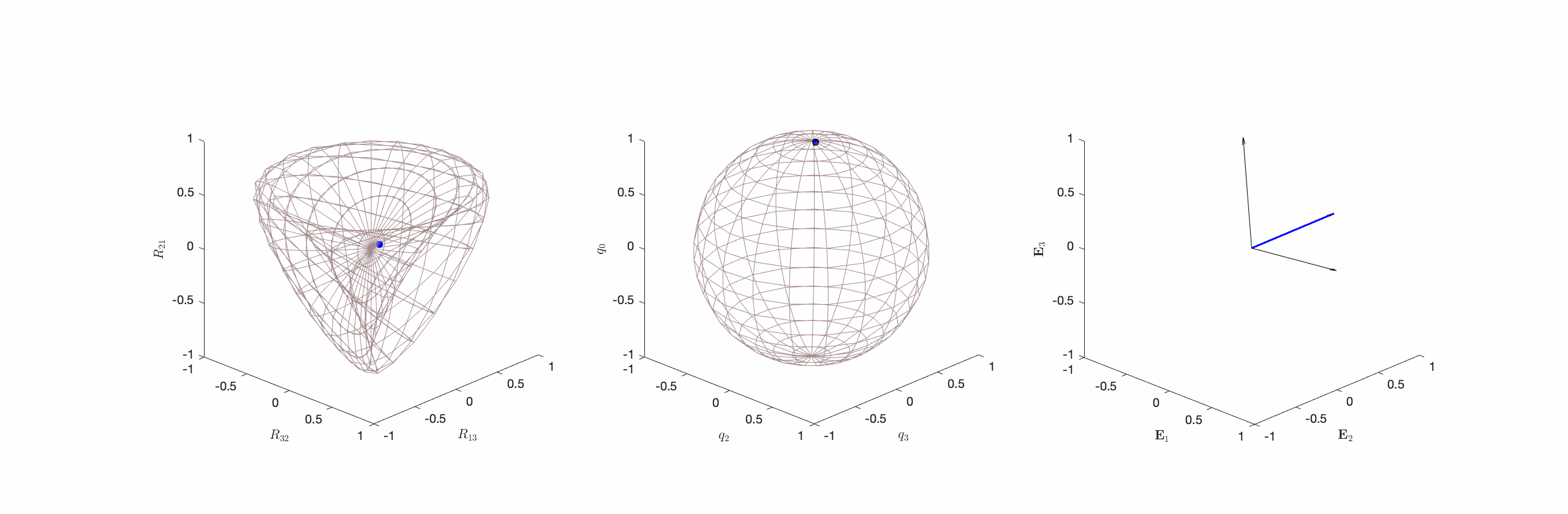 onto appear as circles of unit radii, and (c) the corresponding spherical indicatrices of the instantaneous axis of rotation (shown in blue), axis of rotation (shown in red), and the vectors . The motion of the rigid body corresponding to the Type I motion is best inferred from (c). That is, the rigid body appears to rotate about
  . This figure is adopted from Novelia and O’Reilly [13].
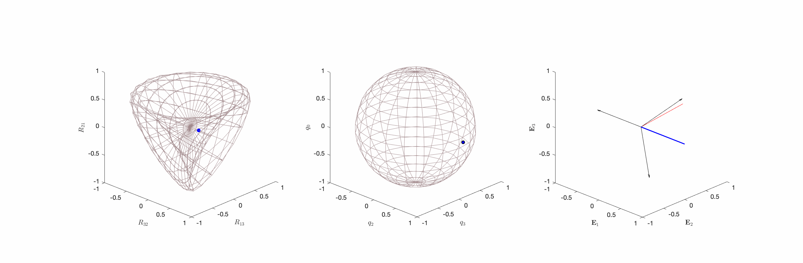 onto appear as a circle of unit radius, and (c) the corresponding spherical indicatrices of the instantaneous axis of rotation (shown in blue), axis of rotation (shown in red), and the vectors . The motion of the rigid body corresponding to the Type II motion is best inferred from (c) by noting that the body will appear to rotate about the instantaneous axis of rotation (shown in blue). This figure is adopted from Novelia and O’Reilly [13].
 onto appear as circles with unit radii, and (c) the corresponding spherical indicatrices of the instantaneous axis of rotation (shown in blue),the axis of rotation (shown in red), and the vectors . The reader should observe that although rotate at constant speed about
  , the axis and angle do not have constant rates of change. The motion of the rigid body corresponding to the Type III motion is best inferred from (c) by noting that the body will appear to rotate about the instantaneous axis of rotation (shown in blue). This figure is adopted from Novelia and O’Reilly [13].
Geodesics of SO(3): alternate measures of distance on SO(3) inspired by axisymmetric and asymmetric rigid bodies
The kinematical line element or measure of distance for the configuration manifold in (17) is the simplest possible and is analogous to considering a spherically symmetric rigid body. However, inspired by the moment-free rotational motion of axisymmetric and asymmetric rigid bodies, alternative metrics are available. As we shall see, for the metrics considered here, Type I and Type II constant angular velocity motions are possible geodesics but motions with non-constant angular velocities are also possible.
In the case of an axisymmetric body, the body possesses two distinct principal moment of inertia  such that
  . The rotational kinetic energy will change accordingly such that
(37) 
where  . The balance of angular momentum for the rigid body is
(38) ![\begin{equation*}\left[ \begin{array}{c}\lambda_t \dot{\omega}_1 \\\lambda_t\dot{\omega}_2 \\\lambda_3 \dot{\omega}_3 \\\end{array} \right] = \left[ \begin{array}{c}- \left( \lambda_3 - \lambda_2 \right) \omega_3\omega_2 = - \left( \lambda_3 - \lambda_{\text{t}} \right) \omega_3\omega_2 \\- \left( \lambda_1 - \lambda_3\right) \omega_3\omega_1 = \left( \lambda_3 - \lambda_{\text{t}} \right) \omega_3\omega_1\\- \left( \lambda_2 - \lambda_1\right) \omega_1\omega_2 = 0\\\end{array} \right]\end{equation*}](https://rotations.berkeley.edu/wp-content/ql-cache/quicklatex.com-9a8ce2ac8f107b936f6b44d5cea43334_l3.png "Rendered by QuickLaTeX.com")
A graphical representation of the solutions to (38) is shown in Figure 9.2(a) of [28]. The solutions conserve the energy and the kinematical line-element for is
(39) 
We note that constant angular velocity motions are possible where  or
or  where are constant. These constant angular velocity motions are geodesics of corresponding to Type I and Type II constant angular velocity motions (cf. Figures 2 and 3)). In addition, geodesics of also include a class of rotations where
  is constant but
  varying periodically in time. An example of one such motion is shown in Figure 5. For this rotational motion, the rigid body no longer executes a simple rotational motion: the third corotational basis vector
  that is parallel to the axis of symmetry for the axisymmetric body traces out a circular path while
  and
and  appears to be far more haphazard.
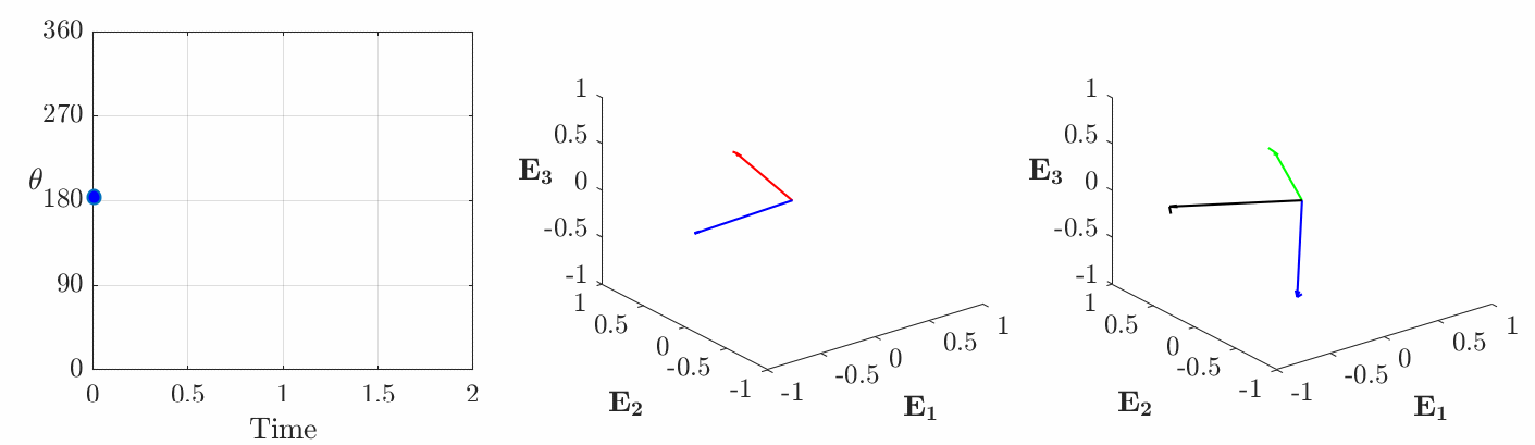
 . (a) The angle of rotation given by the Euler parameter , (b) the instantaneous axis of rotation
  (shown in blue) and the axis of rotation
  (shown in red), (c) trajectories of the corotational basis vectors
  ( (black),
  (green), (blue)). For the results shown in this figure
  and
and  .
.In the case of an asymmetric body, the body possesses three distinct principal moment of inertia  . The rotational kinetic energy has the representation:
(40) 
The balance of angular momentum for the rigid body is
(41) ![\begin{equation*}\left[ \begin{array}{c}\lambda_1 \dot{\omega}_1 \\\lambda_2\dot{\omega}_2 \\\lambda_3 \dot{\omega}_3 \\\end{array} \right] = \left[ \begin{array}{c}- \left( \lambda_3 - \lambda_2 \right) \omega_3\omega_2 \\- \left( \lambda_1 - \lambda_3\right) \omega_3\omega_1 \\- \left( \lambda_2 - \lambda_1\right) \omega_1\omega_2 \\\end{array} \right].\end{equation*}](https://rotations.berkeley.edu/wp-content/ql-cache/quicklatex.com-75156059ab75caf8ab975c768b1e8aa2_l3.png "Rendered by QuickLaTeX.com")
An illustration of the well-known graphical representation of the solutions to (38) is shown in Figure 9.2(b) of [28]. The solutions conserve the energy and the kinematical line-element for is
(42) 
We note that constant angular velocity motions about a principal axis are possible where  where
where  is constant (e.g.,
  ). These constant angular velocity motions are geodesics of corresponding to Type I and Type II constant angular velocity motions (cf. Figures 2 and 3). In addition, geodesics of also include a class of rotations where
  varying periodically in time. An example of one such motion is shown in Figure 6. For this rotational motion, the rigid body no longer executes a simple rotational motion, rather it will appear to tumble in a haphazard manner. Other examples of a geodesic motion for this case can be found in Figures 9.3-9.5 of [28] and the pair of examples of a book tossed in the air and a tumbling T-handle in space (also known as the Dzhanibekov effect) discussed on this website.

 . (a) The angle of rotation given by the Euler parameter , (b) the instantaneous axis of rotation (shown in blue) and the axis of rotation (shown in red), and (c) trajectories of the corotational basis vectors ( (black), (green), (blue)). For the results shown in this figure,
  ,
,  , and
, and  .
.For the results shown in Figures 5 and 6, initial conditions are  and ,
and ,  ,
,  , and
, and  . Thus, with the help of (3) and (5),
(43) 
and the components  of
of  are
are
(44) ![\begin{equation*} \mathsf{Q}\left( t= 0\right) = \left[ \begin{array}{c c c}2 q^2_{1_0} - 1 & 2 q_{1_0}\sqrt{1 - q^2_{1_0}} & 0 \\2 q_{1_0}\sqrt{1 - q^2_{1_0}} & 1 - 2 q^2_{1_0} & 0 \\0 & 0 & -1\end{array} \right]. \end{equation*}](https://rotations.berkeley.edu/wp-content/ql-cache/quicklatex.com-e423fd99a5f25aadafa2af419b0d194c_l3.png "Rendered by QuickLaTeX.com")
References
- Lanczos, C., The Variational Principles of Mechanics, 4th ed., University of Toronto Press, Toronto (1970).
- Ghosh, B., and Wijayasinghe, I., Dynamics of human head and eye rotations under Donders’ constraint. Automatic Control, IEEE Transactions on 57(10), 2478–2489 (2012).
- Haslwanter, T., Mathematics of three-dimensional eye rotations. Vision Research 35(12), 1727–1739 (1995).
- von Helmholtz, H., A Treatise on Physiological Optics, Vol. III. Dover Publications, New York (1962). Translated from the (1910) third German edition and edited by J.P.C. Southall.
- Lamb, H., The kinematics of the eye. Philosophical Magazine Series 6 38(228), 685–695 (1919).
- Liversedge, S.P., Gilchrist, I.D., and Everling, S. (eds.), The Oxford Handbook of Eye Movements. Oxford University Press, Oxford, New York (2011).
- Polpitiya, A., Dayawansa, W., Martin, C., and Ghosh, B., Geometry and control of human eye movements. IEEE Transactions on Automatic Control 52(2), 170–180 (2007).
- Simonsz, H.J., and Tonkelaar, I., 19th Century mechanical models of eye movements, Donders’ law, Listing’s law and Helmholtz’ direction circles. Documenta Ophthalmologica 74(1–2), 95–112 (1990).
- Tweed, D., and Vilis, T., Geometric relations of eye position and velocity vectors during saccades. Vision Research 30(1), 111–127 (1990).
- Westheimer, G., Kinematics of the eye. Journal of the Optical Society of America 47(10), 967–974 (1957).
- Shoemake, K., Animating rotation with quaternion curves, ACM SIGGRAPH Computer Graphics 19(3) 245-254 (1985).
- Novelia, A. N., and O’Reilly, O. M., On the dynamics of the eye: geodesics on a configuration manifold, motions of the gaze direction and Helmholtz’s theorem, Nonlinear Dynamics 80(3) 1303-1327 (2015).
- Novelia, A. N., and O’Reilly, O. M., On geodesics of the rotation group SO(3), Regular and Chaotic Dynamics 20(6) 729-738 (2015).
- O’Reilly, O. M., and Payen, S., The attitudes of constant angular velocity motions, International Journal of Non-Linear Mechanics 41(7) 1–10 (2006).
- Apery, F., Models of the Real Projective Plane: Computer Graphics of Steiner and Boy Surfaces. Vieweg+Teubner Verlag, Wiesbaden (1987).
- Euler, L., Problema algebraicum ob affectiones prorsus singulares memorabile, Novi Commentari Academiae Scientiarum Imperalis Petropolitanae 15 75-106 (1771). The title translates to “An algebraic problem that is notable for some quite extraordinary relations.”
- Rodrigues, O., Des lois géométriques qui régissent les déplacemens d’un système solide dans l’espace, et de la variation des coordonnées provenant de ses déplacements consideérés indépendamment des causes qui peuvent les produire, Journal des Mathématique Pures et Appliquées 5 380–440 (1840).
- Altmann, S. L., Rotations, Quaternions, and Double Groups, Oxford University Press, New York (1986). Reprinted by Dover Publications in 2005.
- Altmann, S. L., Hamilton, Rodrigues, and the quaternion scandal, Mathematics Magazine 62(5) 291–308 (1989).
- Shuster, M. D., A survey of attitude representations, Journal of the Astronautical Sciences 41(4) 439–517 (1993).
- Hamilton, W. R., On a new species of imaginary quantities connected with a theory of quaternions, Proceedings of the Royal Irish Academy 2 424-434 (1844).
- Cayley, A., On certain results relating to quaternions, Philosophical Magazine 26 141–145 (1845). Reprinted in pp. 123–126 of The Collected Mathematical Papers of Arthur Cayley, Sc.D., F.R.S., Vol. 1, Cambridge University Press, Cambridge (1889).
- Gauss, C. F., Mutationen des raumes, in: K. Gesellschaft der Wissenschaften zu Göttingen (ed.), Carl Friedrich Gauss Werke, Vol. 8, pp. 357–362, B. G. Teubner, Leipzig (1900).
- Gray, J. J., Olinde Rodrigues’ paper of 1840 on transformation groups, Archive for History of Exact Sciences 21(4) 375–385 (1980).
- Pujol, J., Hamilton, Rodrigues, Gauss, quaternions, and rotations: A historical reassessment, Communications in Mathematical Analysis 13(2) 1-14 (2012).
- Faruk Senan, A. F., and O’Reilly, O. M., On the use of quaternions and Euler-Rodrigues symmetric parameters with moments and moment potential, International Journal of Engineering Science 47(4) 595-609 (2009).
- Nikravesh, P. E., Wehage, R. A., and Kwon, O. K., Euler parameters in computational kinematics and dynamics. Part 1, ASME Journal of Mechanisms, Transmissions, and Automation in Design 107(3) 358-365 (1985).
- O’Reilly, O. M., Intermediate Dynamics for Engineers: Newton-Euler and Lagrangian Mechanics, 2nd ed., Cambridge University Press, Cambridge (2020).
- O’Reilly, O. M., and Varadi, P. C., Hoberman’s sphere, Euler parameters and Lagrange’s equations, Journal of Elasticity 56(2) 171–180 (1999).
- Demiralp, C., Hughes, J. F., and Laidlaw, D.H., Coloring 3D line fields using Boy’s real projective plane immersion. IEEE Transactions on Visualization and Computer Graphics 15(6),1457–1464 (2009).
- Tu, L. W., An Introduction to Manifolds, 2nd ed., Springer-Verlag, New York (2011).