The double pendulum

Here, we analyze the motions of a planar double pendulum, such as the one illustrated in Figure 1 below. The double pendulum is a fascinating system to examine because of the richness of its chaotic dynamic behavior.

Contents

Equations of motion

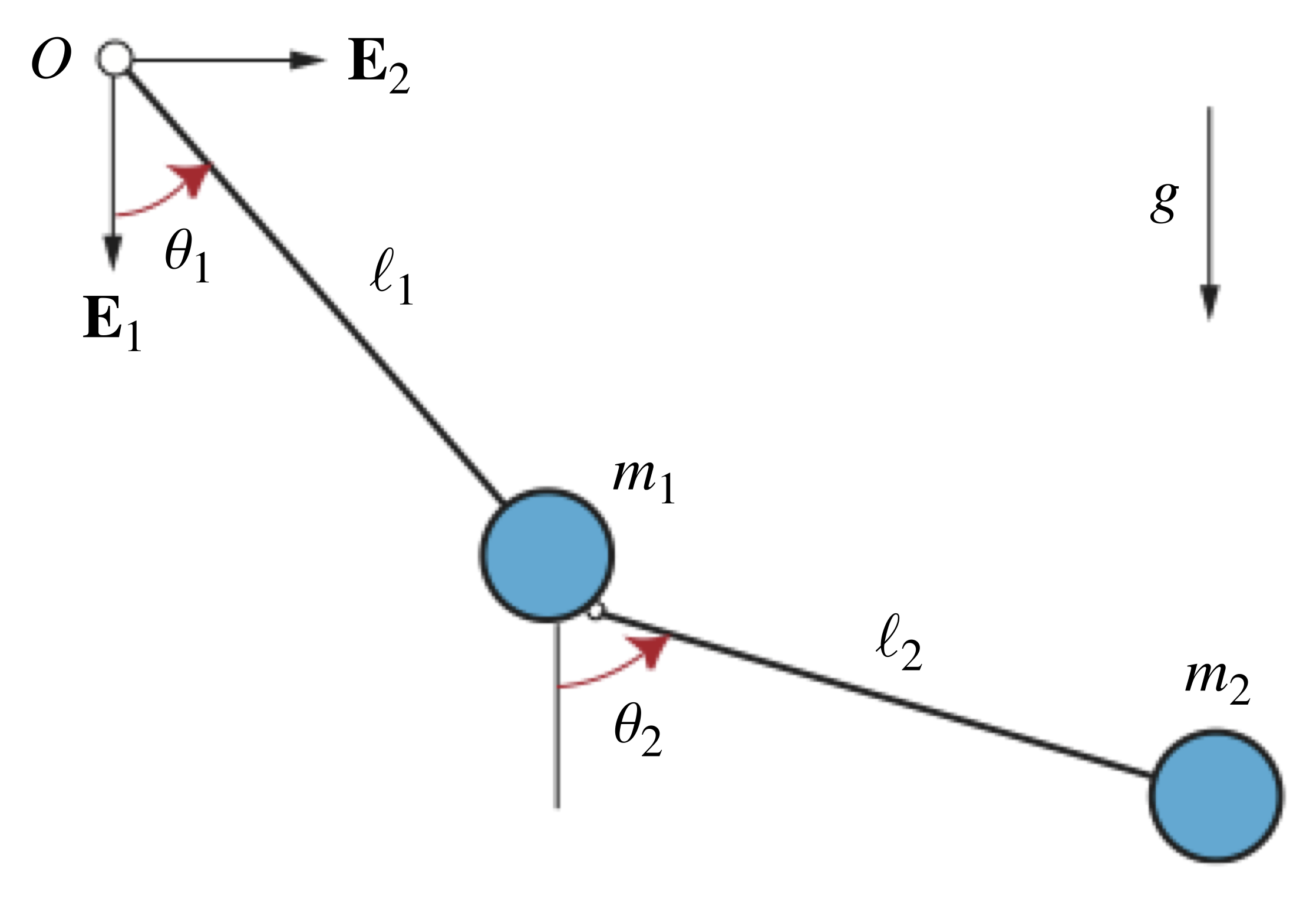
Referring to Figure 1, the planar double pendulum we consider consists of two pendula that swing freely in the vertical plane and are connected to each other by a smooth pin joint, where each pendulum comprises a light rigid rod with a concentrated mass on one end. The first pendulum, whose other end pivots without friction about the fixed origin $O$ , has length $\ell_1$ and mass $m_1$ , while the second pendulum’s length and mass are $\ell_2$ and $m_2$ , respectively. The dynamic behavior of the double pendulum is captured by the angles $\theta_1$ and $\theta_2$ that the first and second pendula, respectively, make with the vertical, where both pendula are hanging vertically downward when $\theta_1 = 0$ and $\theta_2 = 0$ . Consequently, the rotations of the pendula are characterized by the rotation tensors ${\bf L}\left(\theta_1, \, {\bf E}_3\right)$ and ${\bf L}\left(\theta_2, \,{\bf E}_3\right)$ .

**Figure 1.** Schematic of a planar double pendulum.

We can obtain the equations of motion for the double pendulum by applying balances of linear and angular momenta to each pendulum’s concentrated mass or, equivalently, by employing Lagrange’s equations of motion in the form

(1) $\begin{equation*} \frac{\textrm{d}}{\textrm{d}t}\left( \frac{\partial L}{\partial \dot{\theta}_i} \right) - \frac{\partial L}{\partial {\theta}_i} = 0 \quad (i = 1, \, 2), \end{equation*}$

where the Lagrangian $L = T - U$ depends on the double pendulum’s kinetic energy

(2) $\begin{equation*} T = \frac{m_1 + m_2}{2} \ell^2_1 \dot{\theta}^2_1 + \frac{m_2}{2} \ell^2_2 \dot{\theta}^2_2 + m_2 \ell_1 \ell_2 \dot{\theta}_1\dot{\theta}_2 \cos\left(\theta_1 - \theta_2\right) \end{equation*}$

and its potential energy

(3) $\begin{equation*} U = -\left(m_1 + m_2\right) \ell_1 g \cos\left(\theta_1\right) - m_2 \ell_2 g \cos\left(\theta_2\right). \end{equation*}$

Evaluating (1) and then introducing the dimensionless mass, length, and time parameters

(4) $\begin{eqnarray*} && \mu = \frac{m_2}{m_1}, \\ \\ \\ && \lambda = \frac{\ell_2}{\ell_1}, \\ \\ \\ && \tau = \sqrt{\frac{g}{\ell_1}} \ t, \end{eqnarray*}$

respectively, yields the following pair of nondimensional, second-order, ordinary differential equations governing the double pendulum’s behavior:

(5) $\begin{eqnarray*} && (1 + \mu) \theta_{1}^{\prime \prime} + \mu \lambda \left( \theta_{2}^{\prime \prime} \cos \left(\theta_2 - \theta_1 \right) - \left( \theta_{2}^{\prime} \right)^2 \sin \left(\theta_2 - \theta_1 \right) \right) + (1 + \mu) \sin \left(\theta_1\right) = 0, \hspace{1in} \scalebox{0.001}{\textrm{\textcolor{white}{.}}} \\ \\[0.10in] && \mu \lambda^2 \theta_{2}^{\prime \prime} + \mu \lambda \left( \theta_{1}^{\prime \prime} \cos \left(\theta_2 - \theta_1 \right) + \left( \theta_{1}^{\prime} \right)^2 \sin \left(\theta_2 - \theta_1 \right) \right) + \mu \lambda \sin \left(\theta_2\right) = 0 , \end{eqnarray*}$

where the prime symbol denotes differentiation with respect to the dimensionless time $\tau$ . If we arrange the angles $\theta_1$ and $\theta_2$ in a column vector $\mathsf{u} = \left [ \theta_1, \ \theta_2 \right ]^T$ , then the system of differential equations in (5) can be written in the convenient second-order matrix-vector form $\mathsf{M}(\tau, \, \mathsf{u}) \mathsf{u}^{\prime \prime} = \mathsf{f}(\tau, \, \mathsf{u})$ , where

(6) $\begin{eqnarray*} && \mathsf{M}(\tau, \, \mathsf{u}) = \left[ \begin{array}{c c} \left(1 + \mu \right) & \mu \lambda \cos\left(\theta_1 - \theta_2\right) \\ \mu \lambda \cos\left(\theta_1 - \theta_2\right) & \mu \lambda^2 \end{array} \right], \\ \\ \\ && \mathsf{f}(\tau, \, \mathsf{u}) = \left[ \begin{array}{c} - (1+ \mu) \sin \left(\theta_1\right) - \mu \lambda \left( \theta_{2}^{\prime} \right)^2 \sin \left(\theta_1 - \theta_2 \right) \\ -\mu \lambda \sin \left(\theta_2\right) + \mu \lambda \left( \theta_{1}^{\prime} \right)^2 \sin \left(\theta_1 - \theta_2 \right) \end{array} \right]. \end{eqnarray*}$

Before we can numerically integrate the double pendulum’s equations of motion in MATLAB, we must express the equations in first-order form. To do so, we introduce the state vector $\mathsf{y} = \left [ \mathsf{u}^T, \ (\mathsf{u}^{\prime})^T \right ]^T$ such that

(7) $\begin{equation*} \mathsf{y}^{\prime} = \left[\begin{array}{c} \mathsf{u}^{\prime} \\ \mathsf{M}^{-1}(\tau, \, \mathsf{u}) \mathsf{f}(\tau, \, \mathsf{u}) \end{array} \right], \end{equation*}$

which is a form of the equations of motion that is suitable for numerical integration in MATLAB.

Simulation and animation

Provided a set of initial conditions $\theta_i(\tau_0)$ and $\theta_i^{\prime}(\tau_0)$ , we may now numerically compute the evolution of each pendulum’s angular displacement $\theta_i(\tau)$ and then construct the motion of the overall double pendulum. Figure 2 contains the animated behavior of the double pendulum for one such simulation. In this case, the pendulum was dragged into the initial configuration $\theta_1(\tau_0) = 0.8313$ and $\theta_2(\tau_0) = 2.3805$ and then released from rest: $\theta_1^{\prime}(\tau_0) = \theta_2^{\prime}(\tau_0) = 0$ . The parameter values were taken as $\mu = 1$ and $\lambda = 1$ , i.e., the masses and lengths of the pendula were identical: $m_1 = m_2$ and $\ell_1 = \ell_2$ . Also shown in Figure 2 is an animation of the double pendulum’s single-particle representation moving on its so-called configuration manifold, which in this case is a torus parameterized by the angular displacements $\theta_1$ and $\theta_2$ . Casey showed that the response of a system of particles (such as the idealized double pendulum we consider here) can be reduced to the motion of a single representative particle moving on a manifold; we refer the interested reader to Casey’s paper [1] for the details of this single-particle construction. Finally, note that all motions of the double pendulum, regardless of their initial conditions, must conserve the total mechanical energy $E = T + U$ because the pendulum swings freely with no dissipation.

Figure 2. Sample animations of the double pendulum’s response behavior when released from rest and the motion of the corresponding single-particle representation on its configuration manifold, which is a torus.

Downloads

The animations in Figure 2 were generated using the following MATLAB code:

Main script:	Solve the double pendulum’s equations of motion
Supporting files:	Bound the angles to the range (−π, π) Draw a torus for the configuration manifold **

** Many thanks to the late Kermit Sigmon of the University of Florida and to Tim Davis at Texas A&M University for this code.

References

Casey, J., Geometrical derivation of Lagrange’s equations for a system of particles, American Journal of Physics 62(9) 836–847 (1994).