The evolution of the directors

Here, we explicitly show how, with knowledge of the strains for a directed curve and a particular parameterization of a rotation tensor, one may determine the orientation of the curve’s associated directors at each material point by solving a system of ordinary differential equations.

Contents

Equations of motion

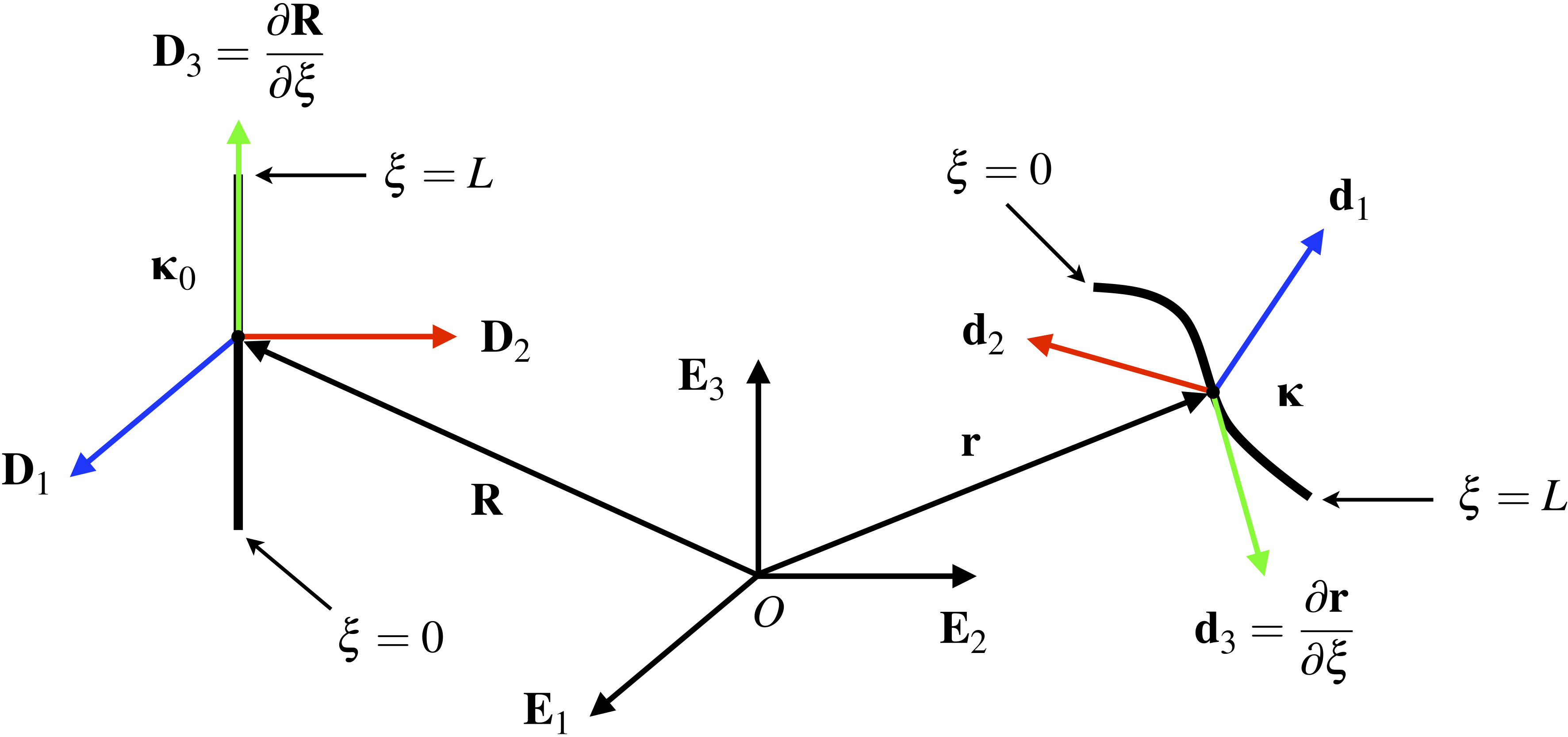
Referring to Figure 1, consider an inextensible material curve of length $L$ with convected coordinate $\xi$ . We define a right-handed orthonormal triad $\{ \mathbf{D}_{1}, \, \mathbf{D}_{2}, \, \mathbf{D}_{3} \}$ at each material point in the curve’s reference configuration $\bkappa_{0}$ . Similarly, we have at each $\xi$ in the curve’s current configuration $\bkappa$ an associated triad $\{ \mathbf{d}_{1}, \, \mathbf{d}_{2}, \, \mathbf{d}_{3} \}$ , where the vectors $\mathbf{d}_{1}$ and $\mathbf{d}_{2}$ are known as directors. Note that the absolute position of a material point on the curve in the reference and current configurations is denoted by $\mathbf{R}$ and $\mathbf{r}$ , respectively, which are expressed in terms of the space-fixed basis $\{ \mathbf{E}_{1}, \, \mathbf{E}_{2}, \, \mathbf{E}_{3} \}$ .

**Figure 1.** Schematic of a directed curve in the reference and current configurations, $\bkappa_{0}$ and $\bkappa$ , respectively.

Recall that according to Kirchhoff’s rod theory, the triads $\{ \mathbf{D}_{1}, \, \mathbf{D}_{2}, \, \mathbf{D}_{3} \}$ and $\{ \mathbf{d}_{1}, \, \mathbf{d}_{2}, \, \mathbf{d}_{3} \}$ at each $\xi$ for the material curve are related such that $\mathbf{d}_{i} = \mathbf{P} \mathbf{D}_{i}$ $(i = 1, \, 2, \, 3)$ , where $\mathbf{d}_{3} = \frac{ \partial \mathbf{r} }{ \partial \xi}$ , $\mathbf{D}_{3} = \frac{ \partial \mathbf{R} }{ \partial \xi}$ , and $\mathbf{P}$ is a rotation tensor. As illustrated in Figure 1, we assume the material curve is undeformed (i.e., it is straight with no pre-twist) in the reference configuration $\bkappa_{0}$ such that $\mathbf{D}_{i} = \mathbf{E}_{i}$ .

Following Love [1], we use a 3-2-3 set of Euler angles $\psi$ , $\theta$ , and $\phi$ to parameterize the rotation tensor $\mathbf{P}$ , and therefore $\mathbf{d}_{i}$ and $\mathbf{E}_{i}$ are related via the matrix-vector expression

(1) $\begin{equation*}\left[ \begin{array}{c c c}\mathbf{d}_{1} \\\mathbf{d}_{2} \\\mathbf{d}_{3}\end{array} \right] =\left[ \begin{array}{c c c }\cos(\phi) & \sin(\phi) & 0 \\- \sin(\phi) & \cos(\phi) & 0 \\0 & 0 & 1\end{array} \right]\left[ \begin{array}{c c c }\cos(\theta) & 0 & -\sin(\theta) \\0 & 1 & 0 \\\sin(\theta) & 0 & \cos(\theta)\end{array} \right]\left[ \begin{array}{c c c }\cos(\psi) & \sin(\psi) & 0 \\- \sin(\psi) & \cos(\psi) & 0 \\0 & 0 & 1\end{array} \right]\left[ \begin{array}{c c c}\mathbf{E}_{1} \\\mathbf{E}_{2} \\\mathbf{E}_{3}\end{array} \right] . \hspace{1in} \scalebox{0.001}{\textrm{\textcolor{white}{.}}}\end{equation*}$

Kirchhoff’s constraints imply that there exists an axial vector

(2) $\begin{equation*}\bnu = \mathrm{ax} \left ( \mathbf{P}^{T} \frac{ \partial \mathbf{P} }{ \partial \xi } \right ) = \mathrm{ax} \left ( \mathbf{K} \right )\end{equation*}$

associated with the skew-symmetric tensor $\mathbf{K} =\sum_{j \, \, = \, 1}^{3} \sum_{k \, \, = \, 1}^{3} K_{kj} \mathbf{E}_{k} \otimes \mathbf{E}_{j}$ , with $K_{kj} = -K_{jk}$ for $j \neq k$ . Consequently, (2) yields

(3) $\begin{equation*}\bnu = K_{32} \mathbf{E}_{1} + K_{13} \mathbf{E}_{2} + K_{21} \mathbf{E}_{3}= \sum_{i \, \, = \, 1}^{3} \nu_{i} \mathbf{E}_{i} , \end{equation*}$

where $\nu_{i} = \nu_{i}(\xi)$ denote strain measures for the material curve; $\nu_{1}$ and $\nu_{2}$ correspond to bending of the curve, while $\nu_{3}$ is associated with torsion. By extracting the $\mathbf{E}_{i}$ components of expression (3), we obtain a system of ordinary differential equations that governs the orientation of the triad $\{ \mathbf{d}_{1}, \, \mathbf{d}_{2}, \, \mathbf{d}_{3} \}$ at every material point on the directed curve. These differential equations may be expressed in the first-order form $\mathsf{M}(\xi, \, \mathsf{y}) \mathsf{y}' = \mathsf{f}(\xi, \, \mathsf{y})$ for numerical integration in MATLAB, where the prime denotes differentiation with respect to the convected coordinate $\xi$ . If we define the state vector $\mathsf{y} = \left [ \psi, \ \theta, \ \phi \right ]^{T}$ , then

(4) $\begin{eqnarray*}&& \mathsf{M}(\xi, \, \mathsf{y}) = \left[ \begin{array}{c c c}-\sin(\theta) \cos(\phi) & \sin(\phi) & 0 \\\sin(\theta) \sin(\phi) & \cos(\phi) & 0 \\\cos(\theta) & 0 & 1\end{array} \right],\\\\\\&& \textrm{\textcolor{white}{---}} \mathsf{f}(\xi, \, \mathsf{y}) =\left[ \begin{array}{c}\nu_{1}(\xi) \\\nu_{2}(\xi) \\\nu_{3}(\xi)\end{array} \right].\end{eqnarray*}$

Thus, by providing the strains $\nu_{i}(\xi)$ and the initial orientation of the directed curve, we may determine the evolution of the Euler angles, and hence the orientation of $\{ \mathbf{d}_{1}, \, \mathbf{d}_{2}, \, \mathbf{d}_{3} \}$ , along the curve. Lastly, because $\mathbf{d}_{3} = \frac{ \partial \mathbf{r} }{ \partial \xi}$ , the shape of the material curve, $\mathbf{r}(\xi)$ , is obtained as follows:

(5) $\begin{equation*} \mathbf{r}(\xi) = \mathbf{r}(0) \, + \int_{0}^{\xi} \mathbf{d}_{3}(s) \, \textrm{d} s . \end{equation*}$

Simulation and animation

For the simulation results that follow, the material curve is $L = 1.5$ m long and begins at the origin: $\mathbf{r}(0) = \mathbf{0}$ . The initial orientation was chosen such that $\psi(0) = 0$ , $\theta(0) = 30^{\circ}$ , and $\phi(0) = 0$ in order to avoid a singularity in the 3-2-3 set of Euler angles.

First, as a check of our numerical simulation, suppose we leave the material curve undeformed, i.e., the strains $\nu_{i} = 0$ . In this case, we expect the triad $\{ \mathbf{d}_{1}, \, \mathbf{d}_{2}, \, \mathbf{d}_{3} \}$ to remain in the same orientation at each material point along the curve. This behavior is verified when we animate the corresponding results from numerical integration; a sample animation is provided in Figure 2. In this and subsequent animations, the directors $\mathbf{d}_{1}$ and $\mathbf{d}_{2}$ are drawn in blue and red, respectively, while the vector $\mathbf{d}_{3}$ is drawn in green, as shown in Figure 1.

**Figure 2.** Animation of the triad $\{ \mathbf{d}_{1}, \, \mathbf{d}_{2}, \, \mathbf{d}_{3} \}$ along an undeformed directed curve: $\nu_{i} = 0$ $(i = 1, \, 2, \, 3)$ .

Next, we may cause the material curve to be in pure bending by prescribing either $\nu_{1} = \textrm{constant} \neq 0$ , $\nu_{2} = 0$ , and $\nu_{3} = 0$ , or $\nu_{1} = 0$ , $\nu_{2} = \textrm{constant} \neq 0$ , and $\nu_{3} = 0$ . The animation in Figure 3 demonstrates the variation in $\{ \mathbf{d}_{1}, \, \mathbf{d}_{2}, \, \mathbf{d}_{3} \}$ along the curve for the case when $\nu_{1} = 1$ , $\nu_{2} = 0$ , and $\nu_{3} = 0$ .

Pure torsion of the material curve is possible if we set $\nu_{1} = 0$ , $\nu_{2} = 0$ , and $\nu_{3} = \textrm{constant} \neq 0$ . For example, when we prescribe $\nu_{1} = 0$ , $\nu_{2} = 0$ , and $\nu_{3} = 9$ , it is clear from the corresponding animation in Figure 4 that the spinning behavior of $\{ \mathbf{d}_{1}, \, \mathbf{d}_{2}, \, \mathbf{d}_{3} \}$ results from the curve having been twisted.

Lastly, we may deform the material curve in more complicated ways by combining bending and torsion, and by specifying strains that vary along the curve. Consider, for example, the material curve depicted in Figure 5 that is subject to both constant bending and torsion: $\nu_{1} = 2$ , $\nu_{2} = 0$ , and $\nu_{3} = 5$ . Consequently, the variation in $\{ \mathbf{d}_{1}, \, \mathbf{d}_{2}, \, \mathbf{d}_{3} \}$ along the curve is more elaborate than the cases of pure bending and pure torsion.

Alternatively, suppose the strains vary along the material curve according to, say, $\nu_{1}(\xi) = \sqrt{\xi}$ , $\nu_{2}(\xi) = \xi$ , and $\nu_{3}(\xi) = \exp(\xi)$ . As shown in Figure 6, the orientation of $\{ \mathbf{d}_{1}, \, \mathbf{d}_{2}, \, \mathbf{d}_{3} \}$ at each material point varies in a more complicated manner than for the simple bending or torsion cases.

Downloads

The animations in Figures 2–6 were generated using the following MATLAB code:

Main script:	Solve the directors’ equations of motion
Supporting files:	Derive the directors’ equations of motion ** Animate the directors’ motion

** Run this code first to obtain the symbolic equations of motion called by the main script. (The Symbolic Math Toolbox is required.) This code needs to be run only once, before the first use of the main script.

References

Love, A. E. H., A Treatise on the Mathematical Theory of Elasticity, 4th ed., Cambridge University Press, Cambridge (1927).