A book tossed in the air

Here, we explore the behavior of a book tossed in the air by developing a model that governs the book’s motion. Through simulation and animation, we wish to confirm the well-known result that rotation about the book’s intermediate principal axis is unstable in the face of rotational perturbations; in contrast, the spin behavior about the book’s other two principal axes is stable. This topic is discussed in various textbooks, such as [1] and [2]. A related scenario involves tossing a tennis racket into the air while giving it an initial angular velocity about an axis parallel to the racket’s face, which causes the racket to flip through 180 $^\circ$ . This phenomenon is explained in [3] and can be observed in the video in Figure 1.

Figure 1. A tennis racket tumbling after being tossed into the air.

Contents

Equations of motion

Referring to Figure 2, we represent the book by a rigid and uniform rectangular prism of mass $m$ , length $\ell$ , width $w$ , and thickness $b$ . The book’s reference configuration is defined such that the book’s mass center $\overline{X}$ is located at the origin and the space-fixed basis $\left\{ {\bf E}_1, \, {\bf E}_2, \, {\bf E}_3\right\}$ is aligned with the book’s principal axes. We locate the mass center $\overline{X}$ relative to the origin using a set of Cartesian coordinates, $x_{i} = \overline{\mathbf{x}} \cdot \mathbf{E}_{i}$ $(i = 1, \, 2, \, 3)$ . The book’s corotational basis $\left\{ {\bf e}_1, \, {\bf e}_2, \, {\bf e}_3\right\}$ is related to the fixed basis by a rotation ${\bf Q}$ such that ${\bf e}_i = {\bf Q}{\bf E}_i$ .

**Figure 2.** Schematic of a book, represented by a rectangular prism, in the reference and current configurations, $\bkappa_0$ and $\bkappa_t$ , respectively. The points labeled 1 through 4 are provided for perspective.

We can obtain the equations of motion governing the translation of the mass center $\overline{X}$ and the book’s orientation by applying balances of linear and angular momenta, respectively. Neglecting the effect of air drag, the only force exerted on the book after being tossed into the air is the weight $-mg{\bf E}_3$ acting at the center of mass, and so a balance of linear momentum yields the system of equations

(1) $\begin{eqnarray*} && m \ddot{x}_1 = 0, \\ \\ && m \ddot{x}_2 = 0, \\ \\ && m \ddot{x}_3 = - m g, \end{eqnarray*}$

while a balance of angular momentum with respect to the mass center gives

(2) $\begin{eqnarray*} && \lambda_{1} \dot \omega_{1} = - (\lambda_{3} - \lambda_{2}) \omega_{2} \omega_{3} , \\ \\ && \lambda_{2} \dot \omega_{2} = - (\lambda_{1} - \lambda_{3}) \omega_{1} \omega_{3} , \\ \\ && \lambda_{3} \dot \omega_{3} = - (\lambda_{2} - \lambda_{1}) \omega_{1} \omega_{2} , \end{eqnarray*}$

where $\omega_{i} = \bomega \cdot \mathbf{e}_{i}$ are the corotational components of the book’s angular velocity $\bomega$ , and $\lambda_i$ are the principal moments of inertia:

(3) $\begin{eqnarray*} && \lambda_1 = \frac{m}{12}\left(w^2 + b^2\right), \\ \\ \\ && \lambda_2 = \frac{m}{12}\left(\ell^2 + b^2\right), \\ \\ \\ && \lambda_3 = \frac{m}{12}\left(\ell^2 + w^2\right). \end{eqnarray*}$

Suppose we use a set of 3-2-1 Euler angles $\psi$ , $\theta$ , and $\phi$ to parameterize the rotation tensor ${\bf Q} = \sum_{i \, \, = \, 1}^3{\bf e}_i\otimes{\bf E}_i$ . In this case, the tensor’s components $Q_{ij}$ $(i, j = 1, \, 2, \, 3)$ , when arranged in a matrix $\left [ Q_{ij} \right ]$ , have the representation

(4) $\begin{equation*} \left[ \begin{array}{c c c} Q_{11} & Q_{12} & Q_{13} \\ Q_{21} & Q_{22} & Q_{23} \\ Q_{31} & Q_{32} & Q_{33} \\ \end{array} \right] = \left[ \begin{array}{c c c } \cos(\psi) & - \sin(\psi) & 0 \\ \sin(\psi) & \cos(\psi) & 0 \\ 0 & 0 & 1 \end{array} \right] \left[ \begin{array}{c c c } \cos(\theta) & 0 & \sin(\theta) \\ 0 & 1 & 0 \\ - \sin(\theta) & 0 & \cos(\theta) \end{array} \right] \left[ \begin{array}{c c c } 1 & 0 & 0 \\ 0 &\cos(\phi) & - \sin(\phi) \\ 0 & \sin(\phi) & \cos(\phi) \end{array} \right]. \hspace{1in} \scalebox{0.001}{\textrm{\textcolor{white}{.}}} \end{equation*}$

Additionally, the corotational angular velocity components $\omega_{i}$ are related to the Euler angles $\psi$ , $\theta$ , and $\phi$ and their rates of change by

(5) $\begin{eqnarray*} && \omega_{1} = -\dot \psi \sin(\theta) + \dot \phi , \\ \\ && \omega_{2} = \dot \psi \cos(\theta) \sin(\phi) + \dot \theta \cos(\phi) , \\ \\ && \omega_{3} = \dot \psi \cos(\theta) \cos(\phi) - \dot \theta \sin(\phi) . \end{eqnarray*}$

Lastly, by introducing the state vector

(6) $\begin{equation*} \mathsf{y} = \left[ \begin{array}{c c c c c c c c c c c c} \!\! \dot x_1, & \!\! \dot x_2, & \!\! \dot x_3, & \!\! x_1, & \!\! x_2, & \!\! x_3, & \!\! \omega_1, & \!\! \omega_2, & \!\! \omega_3, & \!\! \psi, & \!\! \theta, & \!\! \phi \!\! \end{array} \right]^T , \hspace{1in} \scalebox{0.001}{\textrm{\textcolor{white}{.}}} \end{equation*}$

we can express the the governing equations in (1), (2), and (5) for the translation $\overline{\mathbf{x}}(t)$ of the book’s mass center and the book’s orientation $\mathbf{Q}(t)$ in the first-order matrix-vector form $\mathsf{M}(t, \, \mathsf{y}) \dot{\mathsf{y}} = \mathsf{f}(t, \, \mathsf{y})$ for numerical integration in MATLAB, where

(7) $\begin{eqnarray*} && \mathsf{M}(t, \, \mathsf{y}) = \left[ \begin{array}{c c c c c c c c c c c c} m & 0 & 0 & 0 & 0 & 0 & 0 & 0 & 0 & 0 & 0 & 0 \\ 0 & m & 0 & 0 & 0 & 0 & 0 & 0 & 0 & 0 & 0 & 0 \\ 0 & 0 & m & 0 & 0 & 0 & 0 & 0 & 0 & 0 & 0 & 0 \\ 0 & 0 & 0 & 1 & 0 & 0 & 0 & 0 & 0 & 0 & 0 & 0 \\ 0 & 0 & 0 & 0 & 1 & 0 & 0 & 0 & 0 & 0 & 0 & 0 \\ 0 & 0 & 0 & 0 & 0 & 1 & 0 & 0 & 0 & 0 & 0 & 0 \\ 0 & 0 & 0 & 0 & 0 & 0 & \lambda_1 & 0 & 0 & 0 & 0 & 0 \\ 0 & 0 & 0 & 0 & 0 & 0 & 0 & \lambda_2 & 0 & 0 & 0 & 0 \\ 0 & 0 & 0 & 0 & 0 & 0 & 0 & 0 & \lambda_3 & 0 & 0 & 0 \\ 0 & 0 & 0 & 0 & 0 & 0 & 0 & 0 & 0 & -\sin(\theta) & 0 & 1 \\ 0 & 0 & 0 & 0 & 0 & 0 & 0 & 0 & 0 & \cos(\theta) \sin(\phi) & \cos(\phi) & 0 \\ 0 & 0 & 0 & 0 & 0 & 0 & 0 & 0 & 0 & \cos(\theta) \cos(\phi) & -\sin(\phi) & 0 \end{array} \right], \hspace{1in} \scalebox{0.001}{\textrm{\textcolor{white}{.}}} \\ \\ \\ && \mathsf{f}(t, \, \mathsf{y}) = \left[ \begin{array}{c} 0 \\ 0 \\ -mg \\ \dot x_1 \\ \dot x_2 \\ \dot x_3 \\ - (\lambda_{3} - \lambda_{2}) \omega_{2} \omega_{3} \\ - (\lambda_{1} - \lambda_{3}) \omega_{1} \omega_{3} \\ - (\lambda_{2} - \lambda_{1}) \omega_{1} \omega_{2} \\ \omega_{1} \\ \omega_{2} \\ \omega_{3} \end{array} \right]. \end{eqnarray*}$

Simulation and animation

In simulating the book’s behavior when tossed in the air, we take the book to initially be in an unrotated state with its mass center at the origin: $\psi(t_0) = \theta(t_0) = \phi(t_0) = 0$ and $x_i(t_0) = 0$ . The book is launched vertically, in which case $\dot x_1(t_0) = \dot x_2(t_0) = 0$ and $\dot x_3(t_0) > 0$ , and an initial spin is imparted to examine the stability of rotation about each principal axis. Suppose we first toss the book with an initial spin rate $\Omega$ about its longitudinal axis (i.e., its first principal axis) and with small perturbations $\altepsilon << \Omega$ about the other two principal axes: $\omega_1(t_0) = \Omega$ and $\omega_2(t_0) = \omega_3(t_0) = \altepsilon$ . As shown in the animation in Figure 3, the resulting motion, using values of the physical parameters representative of a small textbook, indicates that the tossed book spins stably about this axis. One corner of the book is highlighted with a blue marker to help better visualize the rotation.

Figure 3. Animation of the tossed book’s motion when imparted with a spin largely about its longitudinal axis (i.e., its first principal axis). The book rotates stably about this axis. The animation was recorded at 4x slower speed.

Next, launch the book with a spin largely about its third principal axis, which corresponds to the axis perpendicular to the book’s front and rear covers: $\omega_1(t_0) = \omega_2(t_0) = \altepsilon$ and $\omega_3(t_0) = \Omega$ . The animated response in Figure 4 demonstrates that rotation about this axis is also stable.

Figure 4. Animation of the tossed book’s motion when imparted with a spin largely about its third principal axis, which is perpendicular to the front and rear covers of the book. The book rotates stably about this axis. The animation was recorded at 4x slower speed.

Lastly, impart a spin mostly about the book’s intermediate (i.e., second) principal axis such that $\omega_1(t_0) = \altepsilon$ , $\omega_2(t_0) = \Omega$ , and $\omega_3(t_0) = \altepsilon$ . As expected, and similar to the tennis racket behavior shown in Figure 1, we see from the animation in Figure 5 that the book tumbles in the air instead of stably spinning about this axis.

Figure 5. Animation of the tossed book’s motion when imparted with a spin largely about its intermediate (i.e., second) principal axis. The book begins to tumble in this case, confirming a well-known instability result. The animation was recorded at 4x slower speed.

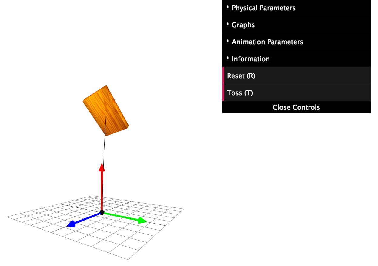
For convenience, an interactive, web-based JavaScript simulation that demonstrates the same behavior animated in Figures 3–5 is accessible through Figure 6.

**Figure 6.** Screenshot of a JavaScript-based book-tossing simulation. Clicking on the above image will open the simulation in a new browser tab; Google Chrome is recommended. We are grateful to Tung Phan for creating this simulation.

Downloads

The MATLAB code used to generate the animations in Figures 3, 4, and 5 is available here.

References

Marsden, J. E., and Ratiu, T. S., Introduction to Mechanics and Symmetry: A Basic Exposition of Classical Mechanical Systems, 2nd ed., Springer-Verlag, New York (1999).
O’Reilly, O. M., Intermediate Dynamics for Engineers: A Unified Treatment of Newton-Euler and Lagrangian Mechanics, Cambridge University Press, Cambridge (2008).
Ashbaugh, M. S., Chicone, C. C., and Cushman, R. H., The twisting tennis racket, Journal of Dynamics and Differential Equations 3(1) 67-85 (1991).