The simplest rotation

To motivate many of our later developments, we start with the simplest case of a rotation: a rotation about a fixed axis ${\bf p}_3$ through an angle $\theta = \theta(t)$ . This example should be familiar to you from many different venues. To describe this rotation, we consider the action of this rotation on the set of fixed, orthonormal, right-handed basis vectors $\left\{ {\bf p}_1, \, {\bf p}_2, \, {\bf p}_3\right\}$ . As depicted in Figure 1, we suppose that these vectors are transformed to the set $\left\{ {\bf t}_1, \, {\bf t}_2, \, {\bf t}_3\right\}$ by the rotation.

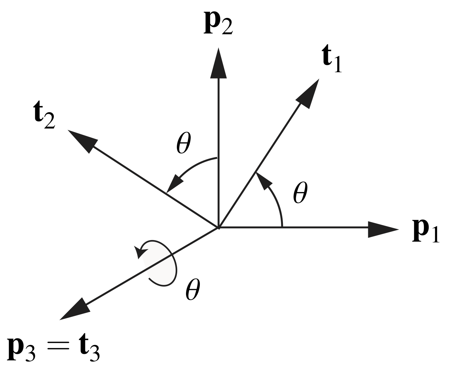
**Figure 1.** The transformation of basis vectors $\left\{ {\bf p}_1, \, {\bf p}_2, \, {\bf p}_3\right\}$ into $\left\{ {\bf t}_1, \, {\bf t}_2, \, {\bf t}_3\right\}$ by a rotation about ${\bf p}_3$ through an angle $\theta$ .

**Figure 1.** The transformation of basis vectors $\left\{ {\bf p}_1, \, {\bf p}_2, \, {\bf p}_3\right\}$ into $\left\{ {\bf t}_1, \, {\bf t}_2, \, {\bf t}_3\right\}$ by a rotation about ${\bf p}_3$ through an angle $\theta$ .

Contents

A matrix representation of the rotation

Using a matrix notation, we can represent the transformation from the set of basis vectors $\left\{ {\bf p}_1, \, {\bf p}_2, \, {\bf p}_3\right\}$ to $\left\{ {\bf t}_1, \, {\bf t}_2, \, {\bf t}_3\right\}$ as

(1) $\begin{equation*} \left[ \begin{array}{c} {\bf t}_1 \\ {\bf t}_2 \\ {\bf t}_3 \end{array} \right] = \underbrace{\left[ \begin{array}{c c c } \cos(\theta) & \sin(\theta) & 0 \\ - \sin(\theta) & \cos(\theta) & 0 \\ 0 & 0 & 1 \end{array} \right]}_{\mathsf{R}} \left[\begin{array}{c} {\bf p}_1 \\ {\bf p}_2 \\ {\bf p}_3 \end{array} \right] . \end{equation*}$

It is easy to see that the matrix $\mathsf{R}$ in (1) has a unit determinant, and its inverse is its transpose: $\mathsf{R}^{-1} = \mathsf{R}^T$ . That is, the matrix $\mathsf{R}$ is proper-orthogonal. By differentiating (1) with respect to time, we find that

(2) $\begin{equation*} \left[ \begin{array}{c} \dot{\bf t}_1 \\ \dot{\bf t}_2 \\ \dot{\bf t}_3 \end{array} \right] = \underbrace{ \dot{\theta} \left[ \begin{array}{c c c } - \sin(\theta) & \cos(\theta) & 0 \\ - \cos(\theta) & - \sin(\theta) & 0 \\ 0 & 0 & 0 \end{array} \right]}_{ \dot{\mathsf{R}} } \left[\begin{array}{c} {\bf p}_1 \\ {\bf p}_2 \\ {\bf p}_3 \end{array} \right]. \end{equation*}$

Using the fact that $\mathsf{R}^{-1} = \mathsf{R}^T$ , we can easily replace ${\bf p}_i$ $(i = 1, \, 2, \, 3)$ in (2) with ${\bf t}_i$ to obtain

(3) $\begin{eqnarray*} \left[ \begin{array}{c} \dot{\bf t}_1 \\ \dot{\bf t}_2 \\ \dot{\bf t}_3 \end{array} \right] \!\!\!\!\! &=& \!\!\!\!\! \underbrace{ \dot{\theta} \left[ \begin{array}{c c c } - \sin(\theta) & \cos(\theta) & 0 \\ - \cos(\theta) & - \sin(\theta) & 0 \\ 0 & 0 & 0 \end{array} \right] }_{ \dot{\mathsf{R}} } \underbrace{ \left[ \begin{array}{c c c } \cos(\theta) & - \sin(\theta) & 0 \\ \sin(\theta) & \cos(\theta) & 0 \\ 0 & 0 & 1 \end{array} \right] }_{ \mathsf{R}^T } \left[\begin{array}{c} {\bf t}_1 \\ {\bf t}_2 \\ {\bf t}_3 \end{array} \right] \hspace{1in} \scalebox{0.001}{\textrm{\textcolor{white}{.}}} \\ \\[0.05in] &=& \!\!\!\!\! \underbrace{\dot{\theta} \left[ \begin{array}{c c c } 0 & 1 & 0 \\ - 1 & 0 & 0 \\ 0 & 0 & 0 \end{array} \right]}_{\dot{\mathsf{R}}\mathsf{R}^T} \left[\begin{array}{c} {\bf t}_1 \\ {\bf t}_2 \\ {\bf t}_3 \end{array} \right]. \end{eqnarray*}$

Notice that this is equivalent to the familiar results $\dot{\bf t}_1 = \dot{\theta}{\bf t}_2$ and $\dot{\bf t}_2 = - \dot{\theta}{\bf t}_1$ from cylindrical polar coordinates. It should also be clear from (3) that $\dot{\mathsf{R}}\mathsf{R}^T$ is a skew-symmetric matrix. A vector $\dot{\theta}{\bf t}_3 = \dot{\theta}{\bf p}_3$ can be introduced that has the useful property that

(4) $\begin{equation*} \dot{\bf t}_k = \dot{\theta}{\bf t}_3 \times {\bf t}_k \quad (k = 1, \, 2, \, 3). \end{equation*}$

You should notice how the vector $\dot{\theta}{\bf t}_3 = \dot{\theta}{\bf p}_3$ can be inferred from the components of $\dot{\mathsf{R}}\mathsf{R}^T$ .

A tensor representation of the rotation

It is convenient to use a tensor notation¹ to describe the rotation we have been discussing. In particular, we can write (1) in the form

(5) $\begin{equation*} {\bf t}_k = {\bf R}{\bf p}_k , \end{equation*}$

where ${\bf R}$ is the tensor

(6) $\begin{equation*} {\bf R} = \cos(\theta)\left( {\bf p}_1\otimes{\bf p}_1 + {\bf p}_2\otimes{\bf p}_2\right) - \sin(\theta)\left( {\bf p}_1\otimes{\bf p}_2 - {\bf p}_2\otimes{\bf p}_1\right) + {\bf p}_3\otimes{\bf p}_3. \hspace{1in} \scalebox{0.001}{\textrm{\textcolor{white}{.}}} \end{equation*}$

It can be shown that this representation of the rotation is equivalent to (1). Furthermore, because

(7) $\begin{eqnarray*} && {\bf I} - {\bf p}_3\otimes{\bf p}_3 = {\bf p}_1\otimes{\bf p}_1 + {\bf p}_2\otimes{\bf p}_2, \\ \\ && {\bf I} - {\bf t}_3\otimes{\bf t}_3 = {\bf t}_1\otimes{\bf t}_1 + {\bf t}_2\otimes{\bf t}_2, \\ \\ && \bepsilon{\bf p}_3 = {\bf p}_1\otimes{\bf p}_2 - {\bf p}_2\otimes{\bf p}_1, \\ \\ && \bepsilon{\bf t}_3 = {\bf t}_1\otimes{\bf t}_2 - {\bf t}_2\otimes{\bf t}_1, \end{eqnarray*}$

we can express the tensor ${\bf R}$ entirely in terms of the axis of rotation ${\bf p}_3 = {\bf t}_3$ and the angle of rotation $\theta$ :

(8) $\begin{equation*} {\bf R} = \cos(\theta)\left( {\bf I} - {\bf p}_3\otimes{\bf p}_3 \right) - \sin(\theta) \left( \bepsilon{\bf p}_3 \right) + {\bf p}_3\otimes{\bf p}_3, \end{equation*}$

or, equivalently,

(9) $\begin{equation*} {\bf R} = \cos(\theta)\left( {\bf I} - {\bf t}_3\otimes{\bf t}_3 \right) - \sin(\theta) \left( \bepsilon{\bf t}_3 \right) + {\bf t}_3\otimes{\bf t}_3. \end{equation*}$

As we shall see later, these equivalent representations naturally lead to the general form of a tensor that represents a rotation about an arbitrary axis through an arbitrary angle of rotation. As with the matrix representation of this simple rotation, the rotation tensor ${\bf R}$ is a proper-orthogonal tensor because it has a determinant of one and its inverse is its transpose: $\mbox{det}\left({\bf R}\right) = 1$ and ${\bf R}^{-1} = {\bf R}^T$ . Differentiating (5), we find that

(10) $\begin{equation*} \dot{\bf t}_k = \dot{\bf R} \underbrace{ {\bf p}_k }_{ {\bf R}^T{\bf t}_k } + \ {\bf R} \underbrace{ {\dot{\bf p}_k} }_{ \mathbf{0} } = \left(\dot{\bf R} {\bf R}^T\right){\bf t}_k , \end{equation*}$

where we have used the fact that ${\bf p}_k$ are constant vectors. Some straightforward computations involving (6) reveal that

(11) $\begin{equation*} \dot{\bf R} = - \dot{\theta}\sin(\theta)\left( {\bf p}_1\otimes{\bf p}_1 + {\bf p}_2\otimes{\bf p}_2\right) - \dot{\theta}\cos(\theta)\left( {\bf p}_1\otimes{\bf p}_2 - {\bf p}_2\otimes{\bf p}_1\right) \hspace{1in} \scalebox{0.001}{\textrm{\textcolor{white}{.}}} \end{equation*}$

and

(12) $\begin{eqnarray*} \dot{\bf R} {\bf R}^T \!\!\!\!\! &=& \!\!\!\!\! \dot{\theta} \left( - {\bf p}_1\otimes{\bf p}_2 + {\bf p}_2\otimes{\bf p}_1\right) \\[0.10in] &=& \!\!\!\!\! \dot{\theta} \left( - {\bf t}_1\otimes{\bf t}_2 + {\bf t}_2\otimes{\bf t}_1\right). \end{eqnarray*}$

With the help of these results, we conclude from (10) that

(13) $\begin{equation*} \dot{\bf t}_k = \left(\dot{\bf R} {\bf R}^T\right){\bf t}_k = \dot{\theta} {\bf t}_3 \times{\bf t}_k . \end{equation*}$

As expected, this result is in agreement with (4). Expression (13) implies that the vector $\dot{\theta} {\bf t}_3 = \dot{\theta} {\bf p}_3$ is the axial vector of the skew-symmetric tensor $\dot{\bf R} {\bf R}^T$ .

Notes

For those unfamiliar with tensor notation, a review of tensors is available in the background section on linear algebra.