We mention here two simple, but intriguing, sequences of rotations that are featured in the Hamilton-Rodrigues theorem and in Codman’s paradox. The compound rotation associated with the latter can be visualized with a sequence of arm motions.
Contents
The Hamilton-Rodrigues theorem
The Hamilton-Rodrigues theorem, which dates to Rodrigues [1] and Hamilton [2] in the mid-19th century, states that a sequence of 180 rotations about three mutually perpendicular axes is equivalent to the identity transformation. To prove this theorem, we first let
  be a set of right-handed orthonormal basis vectors and then use Euler’s representation of a rotation to see that, for a rotation of
  rad about each axis
 ,
,
(1) ![\begin{eqnarray*}{\bf L}\left(\pi, \, {\bf p}_k\right) \!\!\!\!\! &=& \!\!\!\!\! \cos\left(\pi\right)\left( {\bf I} - {\bf p}_k\otimes{\bf p}_k\right) - \sin\left(\pi\right) ( \bepsilon {\bf p}_k ) + {\bf p}_k\otimes{\bf p}_k \hspace{1in} \scalebox{0.001}{\textrm{\textcolor{white}{.}}}\\[0.075in]&=& \!\!\!\!\! - \left( {\bf I} - {\bf p}_k\otimes{\bf p}_k\right) + {\bf p}_k\otimes{\bf p}_k\\[0.075in]&=& \!\!\!\!\! 2{\bf p}_k\otimes{\bf p}_k - {\bf I}.\end{eqnarray*}](https://rotations.berkeley.edu/wp-content/ql-cache/quicklatex.com-83baf4bed7b25be623a1c2625d608da3_l3.png "Rendered by QuickLaTeX.com")
The sequence of rotations of interest is illustrated in Figure 1:  , then
  , followed by
  . That is, the compound rotation is
  .
.
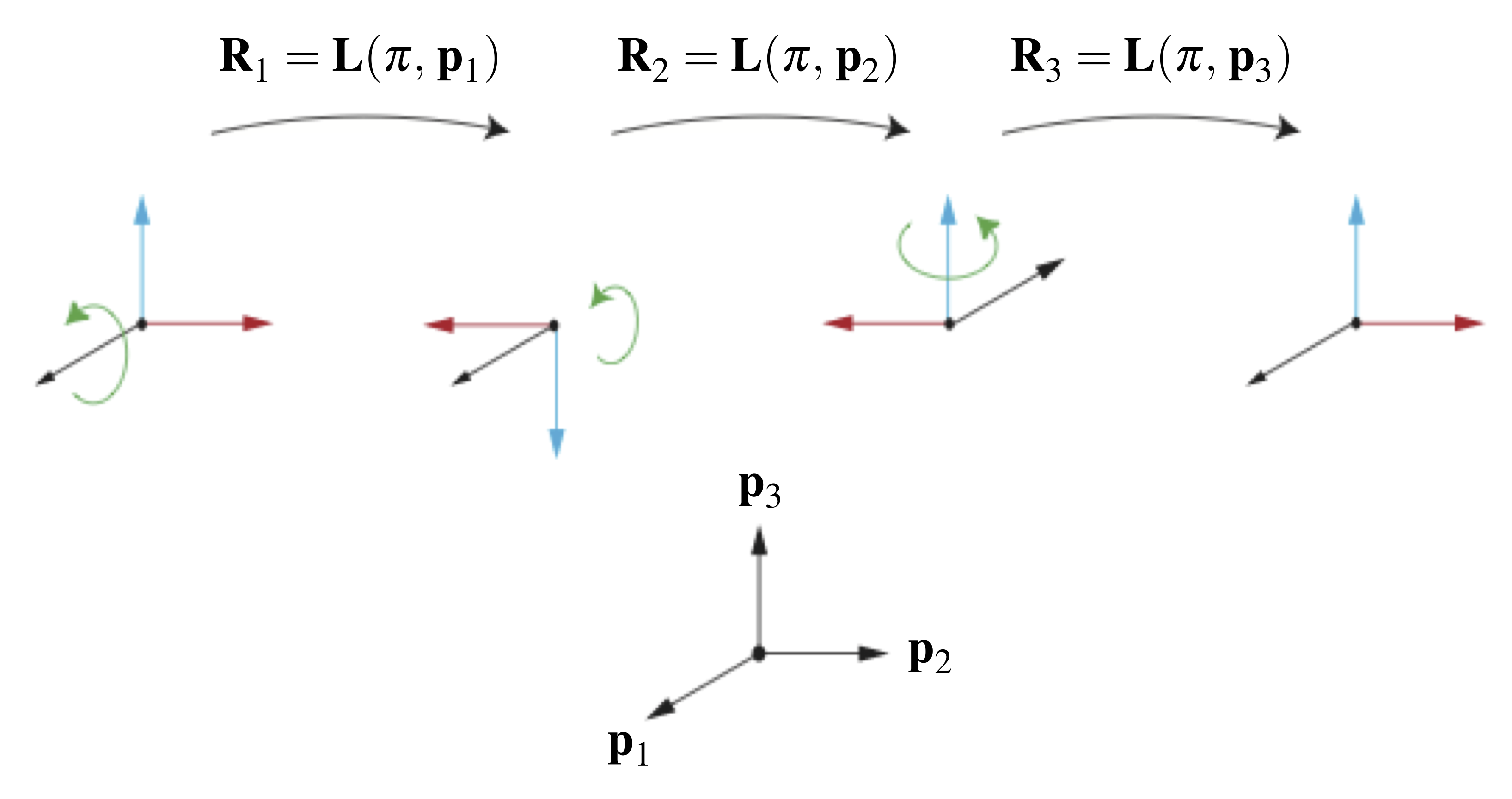
 rad about three mutually perpendicular axes is equivalent to the identity transformation.
With the help of (1), a direct computation shows that the compound rotation
(2) ![\begin{eqnarray*}{\bf L}\left(\pi, \, {\bf p}_3\right){\bf L}\left(\pi, \, {\bf p}_2\right){\bf L}\left(\pi, \, {\bf p}_1\right) \!\!\!\!\! &=& \!\!\!\!\! \left(2 {\bf p}_3\otimes{\bf p}_3 - {\bf I}\right)\left(2 {\bf p}_2\otimes{\bf p}_2 - {\bf I}\right)\left(2 {\bf p_1}\otimes{\bf p}_1 - {\bf I}\right) \hspace{1in} \scalebox{0.001}{\textrm{\textcolor{white}{.}}}\\[0.075in]&=& \!\!\!\!\! \left(2 {\bf p}_3\otimes{\bf p}_3 - {\bf I}\right)\left({\bf I} - 2 {\bf p}_2\otimes{\bf p}_2 - 2 {\bf p_1}\otimes{\bf p}_1\right)\\[0.075in]&=& \!\!\!\!\! {\bf I},\end{eqnarray*}](https://rotations.berkeley.edu/wp-content/ql-cache/quicklatex.com-13626bd296793e412e21c670798706d4_l3.png "Rendered by QuickLaTeX.com")
which proves the theorem. An alternative approach to proving the Hamilton-Rodrigues theorem is presented by Whittaker in Section 3 of [3], in which he uses a purely geometric proof that differs from our algebraic approach above. As shown by Ziegler [4] and further discussed in [5], the Hamilton-Rodrigues theorem can be used to show that a constant moment is not conservative. Additional discussions of conservative moments and moment potentials can be found in [6, 7, 8, 9]. We can also use the theorem to show that a pair of 180 rotations about two perpendicular axes, say,  and
and  , is equivalent to a rotation of 180 about an axis that is mutually perpendicular:
(3) 
Codman’s paradox
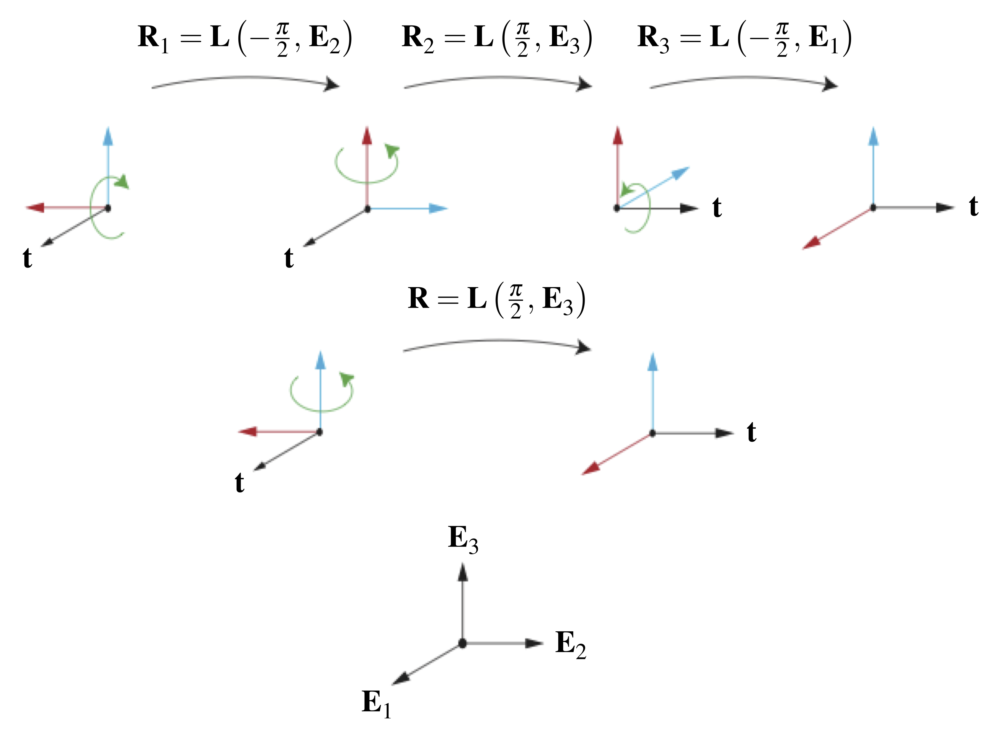
Codman’s paradox features the rotation of the arm about the shoulder joint and dates to 1934 [10]. As quoted from Politti et al. [11], to observe Codman’s paradox, first place your right arm hanging down along your side with your thumb pointing forward and your fingers pointing toward the ground. Next, elevate your arm horizontally so that your fingers point to the right, and then rotate your arm in the horizontal plane so that your fingers now point forward. Finally, rotate your arm downward so that your fingers eventually point toward the ground. After these three rotations, you will notice that your thumb points to the left. That is, your arm rotated by 90. The fact that you get this rotation without having performed a rotation about the longitudinal axis of your arm is known as Codman’s paradox. The sequence of rotations we just described is depicted in Figure 2.
 corresponds to the longitudinal axis of the right thumb.
To explain the 90 rotation observed in Codman’s paradox, we first define a right-handed orthonormal basis  for which
  points up,
  points to the right, and
  points forward, as shown in Figure 2. The first rotation discussed above is a clockwise rotation of 90 about :
(4) 
The second rotation is a 90 counterclockwise rotation about :
(5) 
Lastly, the third rotation is a clockwise rotation of 90 about :
(6) 
Consequently, the compound rotation
(7) ![\begin{eqnarray*}{\bf R}_3{\bf R}_2{\bf R}_1 \!\!\!\!\! &=& \!\!\!\!\! \left({\bf E}_1\otimes{\bf E}_1 - {\bf E}_3\otimes{\bf E}_2 + {\bf E}_2\otimes{\bf E}_3\right)\left({\bf E}_3\otimes{\bf E}_3 - {\bf E}_1\otimes{\bf E}_2 + {\bf E}_2\otimes{\bf E}_1\right){\bf R}_1 \hspace{1in} \scalebox{0.001}{\textrm{\textcolor{white}{.}}}\\[0.075in]&=& \!\!\!\!\! \left(-{\bf E}_1\otimes{\bf E}_2 - {\bf E}_3\otimes{\bf E}_1 + {\bf E}_2\otimes{\bf E}_3\right){\bf R}_1\\[0.075in]&=& \!\!\!\!\! \left(-{\bf E}_1\otimes{\bf E}_2 - {\bf E}_3\otimes{\bf E}_1 + {\bf E}_2\otimes{\bf E}_3\right)\left({\bf E}_2\otimes{\bf E}_2 - {\bf E}_1\otimes{\bf E}_3 + {\bf E}_3\otimes{\bf E}_1\right)\\[0.075in]&=& \!\!\!\!\! -{\bf E}_1\otimes{\bf E}_2 + {\bf E}_3\otimes{\bf E}_3 + {\bf E}_2\otimes{\bf E}_1\\[0.10in]&=& \!\!\!\!\! {\bf L}\left(\frac{\pi}{2}, \, {\bf E}_3\right),\end{eqnarray*}](https://rotations.berkeley.edu/wp-content/ql-cache/quicklatex.com-5f0fb6993b43868ff25323351476ffd7_l3.png "Rendered by QuickLaTeX.com")
or, equivalently,
(8) 
Thus, the sequence of rotations featured in Codman’s paradox is equivalent to a single counterclockwise rotation about the vertical axis by 90, implying that there is no apparent contradiction in Codman’s observations on the behavior of the shoulder joint. This result has an interpretation that can be used to show that successive rotations about three perpendicular axes can be reproduced by a single rotation about one of the axes. A second explanation for the 90 rotation in the motion of the arm discussed earlier is to follow [12] and parameterize the rotation using a set of Euler angles,  . In this case, when the Euler basis vector
  returns to its initial orientation,
  and
and  also return to their initial values, and the relative rotation is the given by the change in
  . It is straightforward to show that this change is
  90. Additional examples of using Euler angles to examine relative rotations can be found in [12].
An extraordinary geometric explanation of Codman’s paradox can be found in Section 123 of Kelvin and Tait’s remarkable Treatise on Natural Philosophy that was first published in 1865 (the same section can be found in the reprinted edition [13]). Kelvin and Tait’s developments were subsequently rediscovered nearly a century later [14] and feature in modern works on geometric phases (see [12, 15] and references therein). Referring to the left-hand panel in Figure 3, consider a unit vector  that corotates with a rigid body, and suppose the motion of the body is such that eventually returns to its original orientation. The locus
  of on the unit sphere encloses a region
  on the sphere’s surface. Kelvin and Tait’s theorem states that, modulo
  , the amount the body has rotated about is equal to the surface area of .

 on the surface of the unit sphere. The panel on the left is used to elucidate Kelvin and Tait’s theorem on relative rotation. The panel on the right shows the locus
  of for the arm motion featured in Codman’s paradox, where points along and corotates with the longitudinal axis of the arm.
To apply Kelvin and Tait’s theorem to examine Codman’s paradox, we refer to the right-hand panel in Figure 3 and imagine the shoulder joint as fixed at the origin of the unit sphere. We trace the locus of , which points from the origin to the finger tips and corotates with the arm. During the arm motion featured in Codman’s paradox, the tip of traces out a spherical triangle on the unit sphere’s surface. The surface area of this triangle occupies  th of the sphere’s total surface area, which is
  . Therefore, the surface area of the triangle is
  , which is identical to the angle of rotation for the compound rotation given in (8).
References
- Rodrigues, O., Des lois géométriques qui régissent les déplacemens d’un système solide dans l’espace, et de la variation des coordonnées provenant de ses déplacements consideérés indépendamment des causes qui peuvent les produire, Journal des Mathématique Pures et Appliquées 5 380–440 (1840).
- Hamilton, W. R., Elements of Quaternions, Chelsea Publishing Company, New York (1967). Edited by C. J. Joly.
- Whittaker, E. T., A Treatise on the Analytical Dynamics of Particles and Rigid Bodies, 4th ed., Cambridge University Press, Cambridge (1937).
- Ziegler, H., Principles of Structural Stability, Blasidell, Waltham, MA (1968). Second edition printed by Birkhäuser in 1977.
- O’Reilly, O. M., Intermediate Dynamics for Engineers: A Unified Treatment of Newton-Euler and Lagrangian Mechanics, Cambridge University Press, Cambridge (2008).
- Antman, S. S., Solution to Problem 71–24, “Angular velocity and moment potentials for a rigid body,” by J. G. Simmonds, SIAM Review 14(4) 649–652 (1972).
- Christoffersen, J., When is a moment conservative?, ASME Journal of Applied Mechanics 56(2) 299-301 (1989).
- Howard, S., Žefran, M., and Kumar, V., On the 6 × 6 Cartesian stiffness matrix for three-dimensional motions, Mechanism and Machine Theory 33(4) 389-408 (1998).
- Simmonds, J. G., Moment potentials, American Journal of Physics 52(9) 851–852 (1984). Errata published on pg. 277 of Vol. 53.
- Codman, E. A., The Shoulder: Rupture of the Supraspinatus Tendon and Other Lesions in or about the Subacromial Bursa, 2nd ed., T. Todd Company, Boston (1934).
- Politti, J. C., Goroso, G., Valentinuzzi, M. E., and Bravo, O., Codman’s paradox of the arm’s rotation is not a paradox: Mathematical validation, Medical Engineering and Physics 20(4) 257–260 (1998).
- O’Reilly, O. M., On the computation of relative rotations and geometric phases in the motions of rigid bodies, ASME Journal of Applied Mechanics 64(4) 969-974 (1997).
- Kelvin, L., and Tait, P. G., Treatise on Natural Philosophy, reprinted ed., Cambridge University Press, Cambridge (1912).
- Goodman, L. E., and Robinson, A. R., Effects of finite rotations on gyroscopic sensing devices, ASME Journal of Applied Mechanics 25 210-213 (1958).
- Marsden, J. E., and Ratiu, T. S., Introduction to Mechanics and Symmetry: A Basic Exposition of Classical Mechanical Systems, 2nd ed., Springer-Verlag, New York (1999).