Here, we discuss how rotations feature in the kinematics of rigid bodies. Specifically, we present various representations of a rigid-body motion, establish expressions for the relative velocity and acceleration of two points on a body, and compare several axes and angles of rotation associated with the motion of a rigid body.
Contents
The motion of a rigid body
A body  is considered to be a collection of material points, i.e., mass particles. Referring to Figure 1, we denote a material point of by, say,
  , and the vector
  locates the material point , relative to a fixed origin
  , at time
  .
.
 and current configuration
  of a body
  . In both configurations, three material points of the body are denoted: ,
  , and
, and  .
.Borrowing from developments in continuum mechanics, we define the current configuration of the body,  , as a smooth, one-to-one, onto function that has a continuous inverse. This function maps a material point of to a point in three-dimensional Euclidean space:
  . We use a subscript to indicate that the function depends on time because the location
  of the particle varies with time. It is important to note that defines the state of the body at time . We also establish a fixed reference configuration of the body,
  . This configuration is defined by the invertible function
  , and thus we may use the position vector
  of in the reference configuration to uniquely define the material point. As a result, using the reference configuration, we can then define the motion of the body as a function of and :
(1) 
Notice that the motion of a material point of depends on the particular material point and instant of time.
Euler’s theorem
For a rigid body, the nature of the motion function (1) can be simplified dramatically. First, the distance between any two material points, say,  and
and  , of a rigid body remains constant for all motions. That is,
(2) 
Second, the rigid body’s motion preserves orientations. Specifically, in 1775, Euler showed that the motion of a body that satisfies (2) is such that
(3) 
where  is a rotation tensor. Recall that has an associated axis and angle of rotation. If we assume that one point of the body is fixed, then we can simplify (3) by choosing the fixed point to be the origin, in which case
(4) 
Thus, from (4), we can then infer Euler’s theorem on the motion of a rigid body:
Every motion of a rigid body about a fixed point is a rotation about an axis through the fixed point.
The axis referred to here is the rotation axis of the tensor  . Because the motion of the body in question is from the reference configuration to the current configuration , this axis depends on the choice of reference configuration. We can arrive at an alternative, and more common, interpretation of Euler’s theorem that does not feature the reference configuration . To do this, we consider the motion of the body with a fixed point during the time interval
 ![\left[t_0, \, t\right]](https://rotations.berkeley.edu/wp-content/ql-cache/quicklatex.com-0cdd7eee1c56608edcb62153a5ab3f1d_l3.png "Rendered by QuickLaTeX.com") , where we emphasize that, for the motion at hand, the body’s configuration changes from the initial state
, where we emphasize that, for the motion at hand, the body’s configuration changes from the initial state  to the current configuration . In this case, we find from (4) that
(5) 
Thus, the motion of the body at the end of the time interval is characterized by the rotation tensor  that, in general, has an axis and angle of rotation that differ from those associated with
  . Invoking Euler’s theorem, the rotation axis of the tensor is the axis of rotation for the motion of the rigid body.
Representations for the general motion
A general motion of a rigid body is one in which the body may not have a fixed point. In this case, it is easy to argue that a uniform translation of the reference configuration can be imposed on the rigid body such that any one of its material points, say,  , is placed at its location
  in the current configuration . The rigid body is then rotated about so as to occupy its current configuration:
(6) 
(7) 
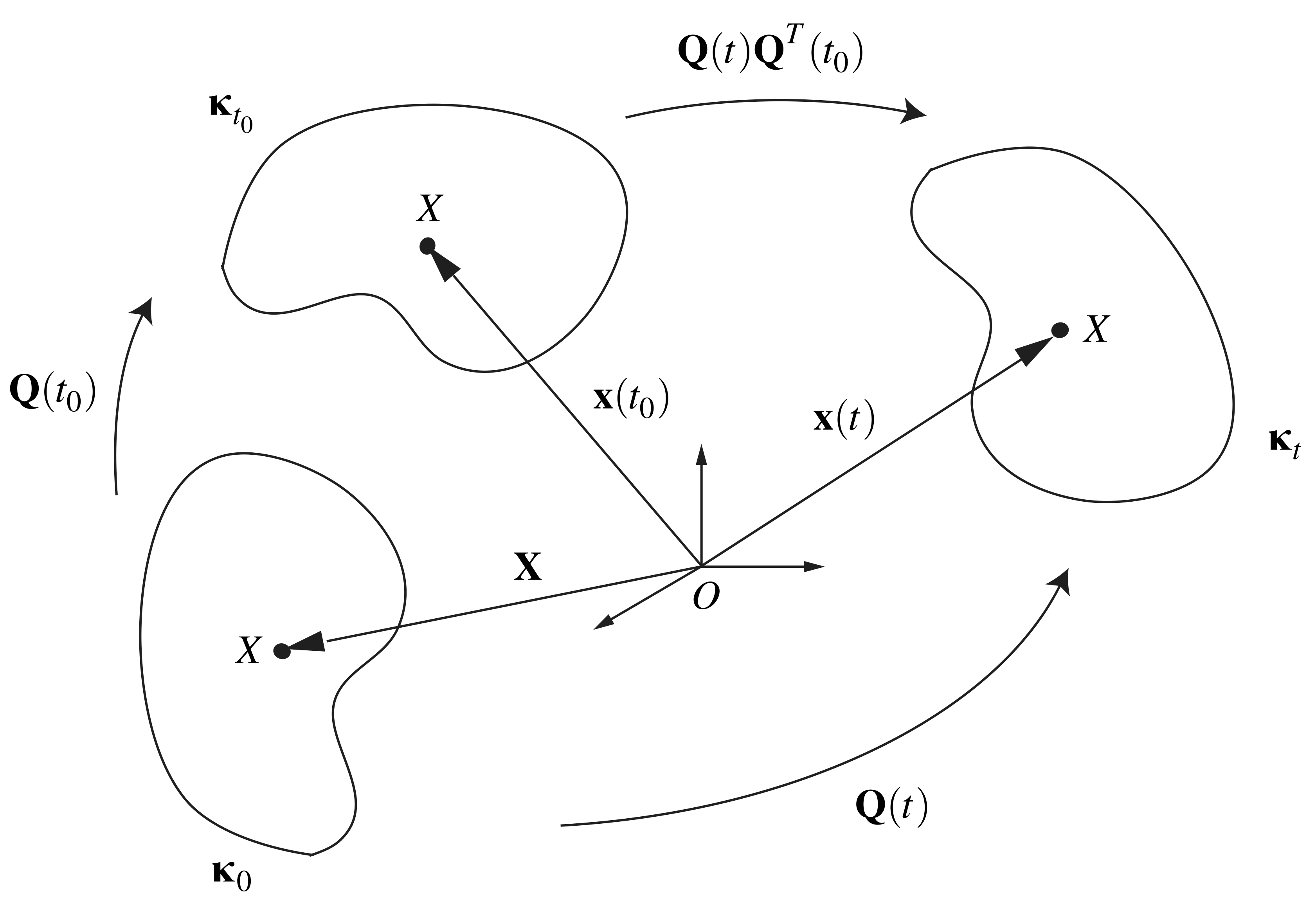
where  . In words, (7) states that the most general motion of a rigid body is a combination of a translation and a rotation. Not surprisingly, this result was also known to Euler [1, 2]. To discuss an alternative to (7) that does not feature the reference configuration , we consider the motion of the body during a time interval
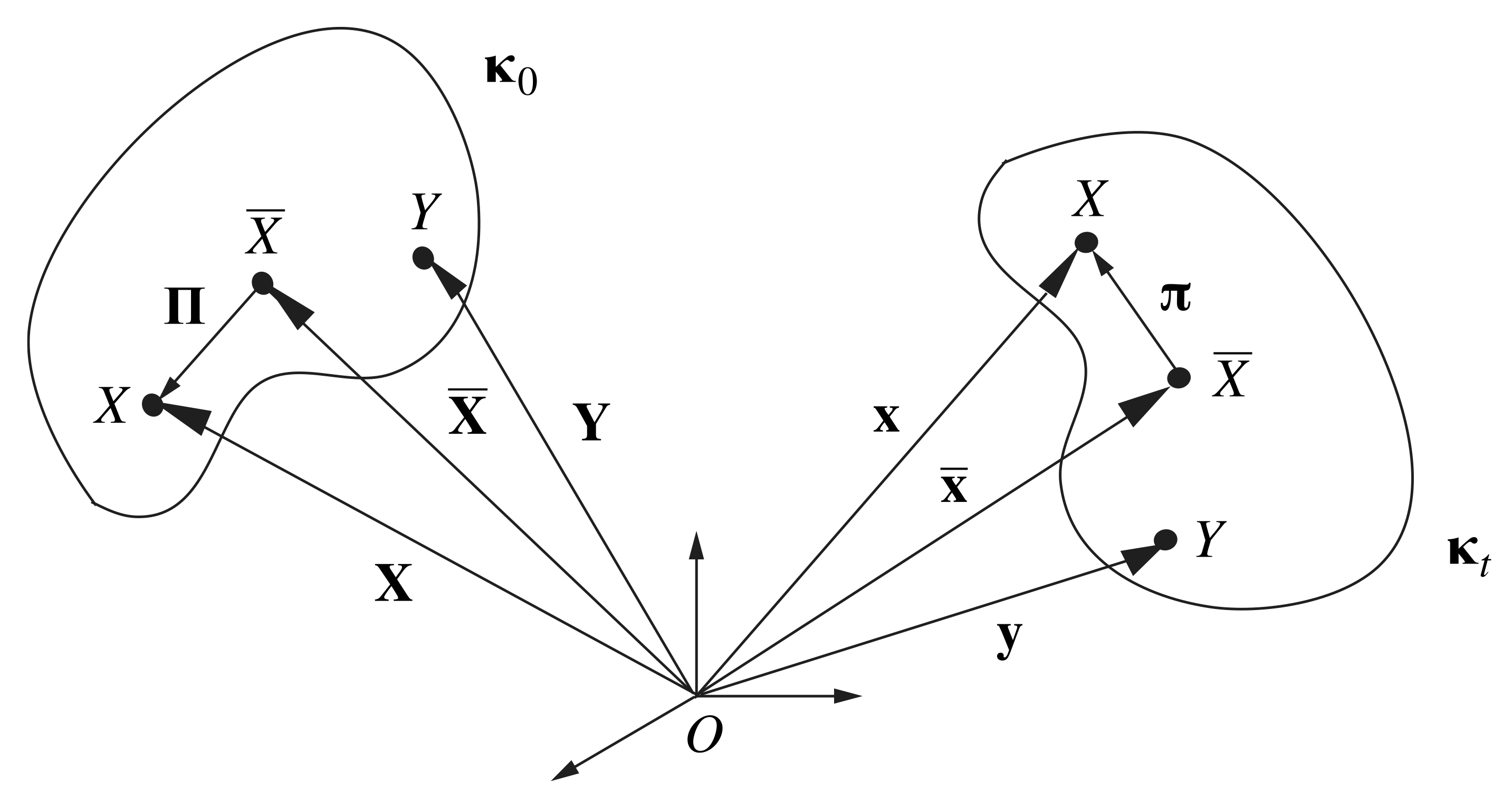
 ![\left[ t_0, \, t\right]](https://rotations.berkeley.edu/wp-content/ql-cache/quicklatex.com-6a7acadedc14044654aae0ea0bb3a913_l3.png "Rendered by QuickLaTeX.com") , as illustrated in Figure 2.
, as illustrated in Figure 2.
 and current configuration
  . Also shown are the reference configuration and illustrations of the roles played by several rotation tensors in the body’s motion.
With the help of (7), we find that
(8) 
Combining (7) and (8), we arrive at an alternative representation of a general rigid-body motion:
(9) 
where  1. Another alternative, synonymous with a famous theorem credited to Michel Chasles (1793–1880) [3], represents the motion of a rigid body by a screw motion. That is, the motion, as shown in Figure 3, is decomposed into a rotation through an angle
  about an axis
  , followed by a translation of
  along that axis.
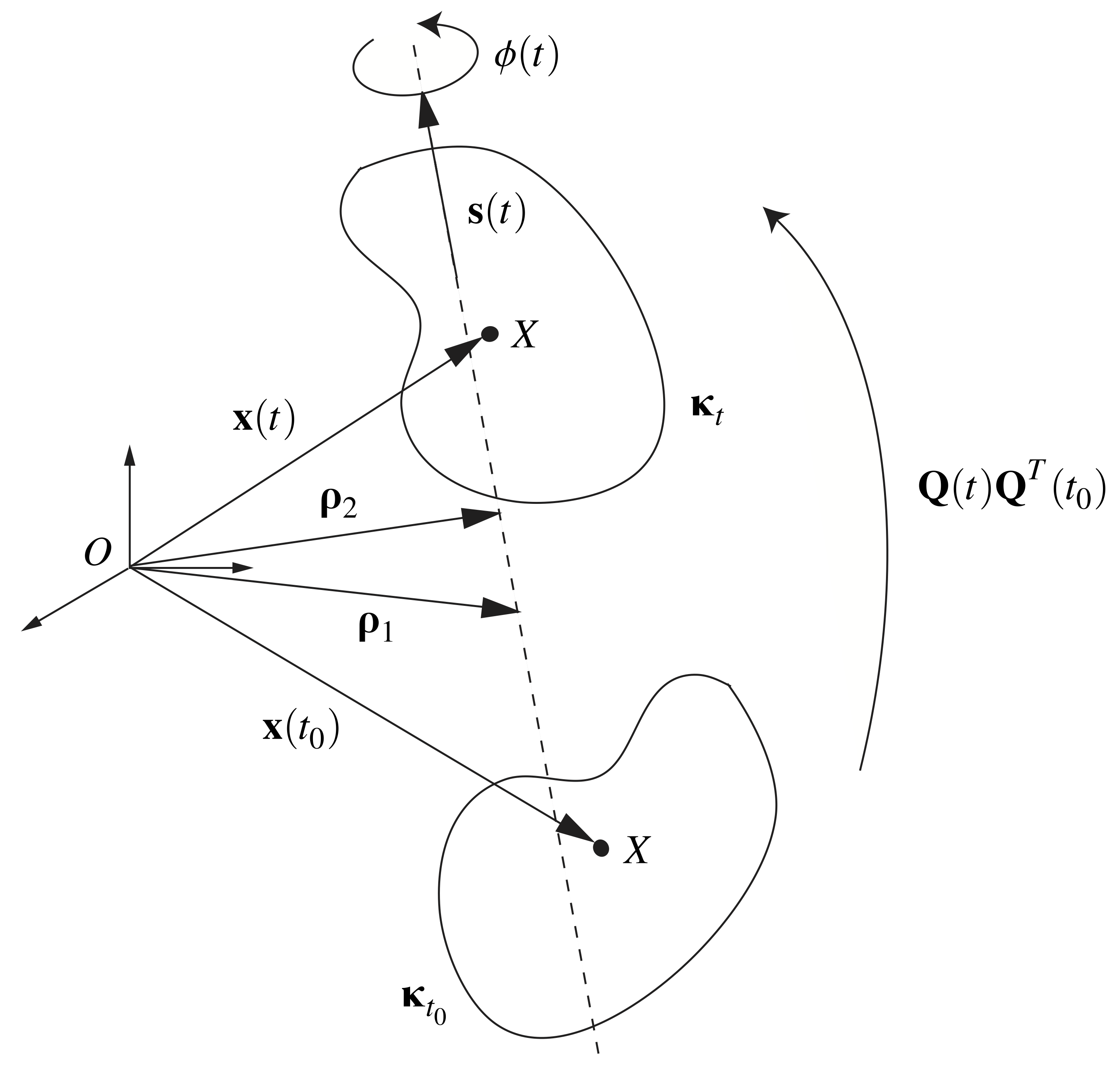 and current configuration of a rigid body depicting the screw axis
  and angle of rotation
  . Here, the rigid body is rotated about through and then translated along the screw axis by an amount
  . Two possible choices of the screw axis intercept
  are also shown. For the first option,
  is chosen to be the intercept of the screw axis with the horizontal plane; for the second,
  is the vector from the origin that intersects the screw axis at a right angle:
  .
.The screw axis and the angle correspond to the rotation axis and angle, respectively, of the rotation tensor  :
:
(10) 
In principle, the body’s translation along the screw axis and the location  of the intercept of the screw axis can be determined from
  , as defined in (9), according to
(11) 
However, the tensor  in (11) is not invertible2. Consequently, is not uniquely defined. Several choices of can be found in the literature, and two choices are depicted in Figure 3. For example, choosing to be normal to the screw axis leads to the following solutions for and :
(12) ![\begin{eqnarray*}&& \sigma(t) = {\bf z}(t)\cdot{\bf s}(t),\\\\[0.10in]&& {\brho}(t) = \frac{1}{2}\left( {\bf z}_\perp(t) + \cot\left( \frac{\phi(t)}{2}\right) {\bf s}(t)\times{\bf z}(t) \right), \end{eqnarray*}](https://rotations.berkeley.edu/wp-content/ql-cache/quicklatex.com-837b43ff53b5b2daf0b1606646c75b4e_l3.png "Rendered by QuickLaTeX.com")
where
(13) 
Finally, note that a special case of the solution to (11) occurs when  , causing to be indeterminate. However, it is still possible to compute using (12)1.
Relative velocity and acceleration
Given representations (7) and (9) for a general rigid-body motion, we can define angular velocity vectors associated with their respective rotation tensors, and  . Conveniently, as
  , both representations have the same angular velocity tensor
  , and hence the same angular velocity vector
  :
:
(14) ![\begin{eqnarray*}{\bOmega} \!\!\!\!\! &=& \!\!\!\!\! \dot{\overline{{\bf Q}(t) {\bf Q}^T(t_0)}} \left({\bf Q}(t) {\bf Q}^T(t_0) \right)^T \\[0.075in]&=& \!\!\!\!\! \dot{\bf Q}(t) \left({\bf Q}(t_0) {\bf Q}^T(t_0) \right) {\bf Q}^T(t)\\[0.075in]&=& \!\!\!\!\! \dot{\bf Q}(t){\bf Q}^T (t) ,\\\\{\bomega} \!\!\!\!\! &=& \!\!\!\!\! \mbox{ax} (\bOmega).\end{eqnarray*}](https://rotations.berkeley.edu/wp-content/ql-cache/quicklatex.com-72b2fcac7429aa3c2671caa2ae57ce11_l3.png "Rendered by QuickLaTeX.com")
Recall that the rotation tensor , and therefore its angular velocity vector  , can be represented in a variety of manners, for instance, using Euler’s representation, a set of Euler angles, the Euler-Rodrigues symmetric parameters (i.e., unit quaternions), etc. Differentiating (3) and utilizing (14), we can obtain an expression for the relative velocity of any two material points of a rigid body, and , in terms of its angular velocity and the relative position of the points:
(15) ![\begin{eqnarray*}{\bf v}_1 - {\bf v}_2 \!\!\!\!\! &=& \!\!\!\!\! \dot{\bf x}_1 - \dot{\bf x}_2= \dot{\bf Q}\left( {\bf X}_1 - {\bf X}_2 \right)= \left( \dot{\bf Q}{\bf Q}^T \right ){\bf Q}\left( {\bf X}_1 - {\bf X}_2 \right)= {\bOmega}\left( {\bf x}_1 - {\bf x}_2 \right) \hspace{1in} \scalebox{0.001}{\textrm{\textcolor{white}{.}}}\\[0.075in]&=& \!\!\!\!\! {\bomega}\times\left( {\bf x}_1 - {\bf x}_2 \right).\end{eqnarray*}](https://rotations.berkeley.edu/wp-content/ql-cache/quicklatex.com-1f3788e124a396d2e31154c26c1dd182_l3.png "Rendered by QuickLaTeX.com")
The body’s angular acceleration  is given by the derivative of :
(16) 
Therefore, from differentiating (15), we find that the relative acceleration can be expressed in terms of , , and the relative position of and :
(17) ![\begin{eqnarray*}{\bf a}_1 - {\bf a}_2 \!\!\!\!\! &=& \!\!\!\!\! \dot{\bf v}_1 - \dot{\bf v}_2= \dot{\bomega}\times\left( {\bf x}_1 - {\bf x}_2 \right)+ {\bomega}\times\left( \dot{\bf x}_1 - \dot{\bf x}_2 \right) \\[0.075in]&=& \!\!\!\!\! {\balpha}\times\left( {\bf x}_1 - {\bf x}_2 \right)+ {\bomega}\times\left( \bomega \times \left( {\bf x}_1 - {\bf x}_2 \right ) \right).\end{eqnarray*}](https://rotations.berkeley.edu/wp-content/ql-cache/quicklatex.com-56c8c9a579f773d611ebacae0b1a37fa_l3.png "Rendered by QuickLaTeX.com")
A corotational basis
Dating to the 18th century, the convenience of using a corotational (or body-fixed, or embedded) basis in rigid-body dynamics has been appreciated. Here, we discuss such a basis and point out some features of its use. It is of interest to note how the basis can be used to define a transparent representation for the rotation tensor of a body. Our discussion of the corotational basis follows Casey [4] with some minor changes.
It is well known that knowledge of the position vectors of three material points suffices to determine the motion of a rigid body. Indeed, this is the premise for optical tracking schemes and is the motivation for our construction of a corotational basis. Referring to Figure 4, we start by picking three material points of a body: , , and  . These points, located relative to an origin by the position vectors
  ,
,  , and
, and  in the body’s reference configuration , are chosen such that orthonormal vectors
  and
and  point from
  toward
  and
and  , respectively:
  and
and  . We then complete the fixed, right-handed Cartesian basis by defining
  .
.

 for a rigid body in its reference configuration and the corotational basis
  in the body’s current configuration .
Now consider the current locations of the three material points, denoted by  ,
,  , and
, and  , after a motion of the body. Because the rotation tensor preserves lengths and orientations, the relative position vectors
  and
and  will retain their relative orientation and lengths. Consequently, using (3), we can establish two orthonormal members of a corotational basis by choosing them to point from toward and , respectively:
  and
and  . We then define
  to complete the basis. Therefore, in terms of the fixed basis
  and the corotational basis
  , the rotation tensor has the simple representation
(18) 
Because the corotational basis moves with the body, we can use our previous results (15) and (17) for the relative velocity and acceleration vectors of two material points on a rigid body to see that the basis vectors differentiate such that
(19) 
Alternatively, we can differentiate the identity  and perform some minor rearranging to obtain the same results. For example,
(20) 
Any vector  can be expressed in terms of the corotational basis because the basis spans
  :
:
(21) 
When the vector components  are constant, is known as a corotational vector. The time derivative of has the representations
(22) ![\begin{eqnarray*}\dot{\bf r} \!\!\!\!\! &=& \!\!\!\!\! \sum_{i \, \, = \, 1}^3 \dot{r}_i {\bf e}_i + \sum_{i \, \, = \, 1}^3 r_i \dot{\bf e}_i \\[0.15in]&=& \!\!\!\!\! \corot{\bf r} + {\bomega}\times{\bf r},\end{eqnarray*}](https://rotations.berkeley.edu/wp-content/ql-cache/quicklatex.com-7a8349f8e16bfd139545707a9b07ec65_l3.png "Rendered by QuickLaTeX.com")
where  is the corotational derivative of . An additional differentiation yields
(23) ![\begin{eqnarray*}\ddot{{\bf r}} \!\!\!\!\! &=& \!\!\!\!\! \sum_{i \, \, = \, 1}^3 \ddot{r}_i {\bf e}_i + 2 \sum_{i \, \, = \, 1}^3 \dot{r}_i \dot{\bf e}_i+ \sum_{i \, \, = \, 1}^3 {r}_i \ddot{\bf e}_i\\[0.15in]&=& \!\!\!\!\! \ccorot{\bf r} +2 \bomega\times\corot{\bf r} + {\balpha}\times{\bf r} + \bomega\times\left({\bomega}\times{\bf r}\right). \end{eqnarray*}](https://rotations.berkeley.edu/wp-content/ql-cache/quicklatex.com-0ca051c7fb6eac62ef74601bd46d5dbf_l3.png "Rendered by QuickLaTeX.com")
The presence of the Coriolis acceleration  in (23) arises because we have chosen to express in a basis that is not fixed. Note that if is a corotational vector, then
  , and the Coriolis acceleration vanishes.
Axes of rotation
It is possible to define three distinct axes of rotation for a rigid body. These axes are commonly used in mechanics and navigation, and to discuss them it is convenient to recall the representations (7) and (9) for a rigid-body motion. The rotation tensor associated with (7) has an axis of rotation  and an angle of rotation
  , while the screw axis and angle are the axis and angle of rotation, respectively, of the rotation tensor for (9). A third rotation axis, known as the instantaneous axis of rotation
  , can also be defined. This axis is a unit vector parallel to the angular velocity vector :
(24) 
Except in the simple case when is constant, the instantaneous axis  does not have an associated angle of rotation. The terminology “instantaneous axis” can be appreciated from the observation that
  for any corotational vector . Thus, if is constant, then will appear to rotate about , as shown in Figure 5. Our definition of the instantaneous axis of rotation is identical to that used in classical works on rigid-body dynamics, such as Poinsot’s text [5] and Sections 405–406 of Poisson’s text [6]. This definition is not universally adapted. For example, in the literature on the kinematics of anatomical joints, the instantaneous axis of rotation often refers to
  and not 3.
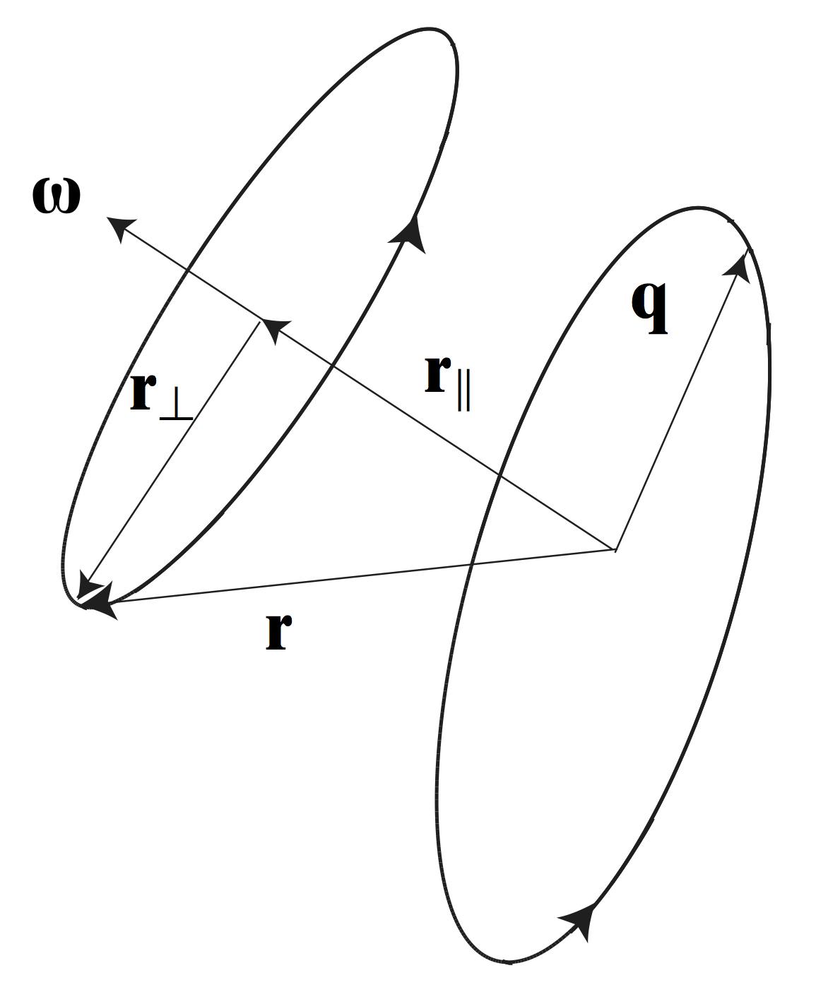
 associated with a rigid-body motion for which
  is constant. In this figure,
  and
and  , and the instantaneous axis of rotation is parallel to . The evolution of another possible rotation axis
  is also shown.
In general, the rotation axes  , , and are not identical. However, we can relate these axes and the two angles of rotation,
  and
and  , through the angular velocity vector :
(25) ![\begin{eqnarray*}{\bomega} \!\!\!\!\! &=& \!\!\!\!\! \dot{\theta}{\bf q} + \sin(\theta)\dot{\bf q}+ (1 - \cos(\theta)){\bf q}\times\dot{\bf q} \\[0.075in]&=& \!\!\!\!\! \dot{\phi}{\bf s} + \sin(\phi)\dot{\bf s} + (1 - \cos(\phi)){\bf s}\times\dot{\bf s}\\[0.075in]&=& \!\!\!\!\! \lnorm \bomega \rnorm {\bf i} .\end{eqnarray*}](https://rotations.berkeley.edu/wp-content/ql-cache/quicklatex.com-27dc8a5b934b1655a3d09b5199c76adb_l3.png "Rendered by QuickLaTeX.com")
In the course of examining the rotation tensors from various problems in rigid-body dynamics, it is straightforward to numerically compute the axes of rotation , , and given a body’s reference configuration, rotation tensor , and angular velocity vector  . In these problems, you will typically find examples in which the axes , , and are distinct. It is, however, also of interest to consider examples for which some of these axes are equal. For instance, suppose a body’s rotation tensor describes a steady rotation about a fixed vertical axis
  through an angle
  at a constant rate
  :
:
(26) 
In this case, it is easy to compute that  and
and  . Now consider an example in which describes a rotation about a time-varying axis of rotation at a constant speed4:
(27) 
where the axis of rotation
(28) ![\begin{eqnarray*}&& {\bf q}(t) = \cos\left(\frac{\nu}{2}\right){\bf E}_1 + \sin\left(\frac{\nu}{2}\right){\bf E}_2, \\\\[0.10in]&& \nu(t) = \dot{\nu}_0 \left(t - t_0\right) + \nu_0,\end{eqnarray*}](https://rotations.berkeley.edu/wp-content/ql-cache/quicklatex.com-e0692fe079f12150fdc287d3c5415c3c_l3.png "Rendered by QuickLaTeX.com")
and  and
and  are constants. Consequently, the angular velocity vector
  , and the angle of rotation
  rad. A standard calculation also reveals that
(29) 
That is, the rotation tensor  corresponds to a rotation about through an angle
  . For this example, it now follows that
(30) 
Indeed, (27) is the simplest example of a rotation that we know of for which the angular velocity is constant but the rotation axis is not parallel to . The temporal behavior of the corotational basis vectors  , the axes of rotation, and the rotation angles and
  are illustrated in Figure 6.
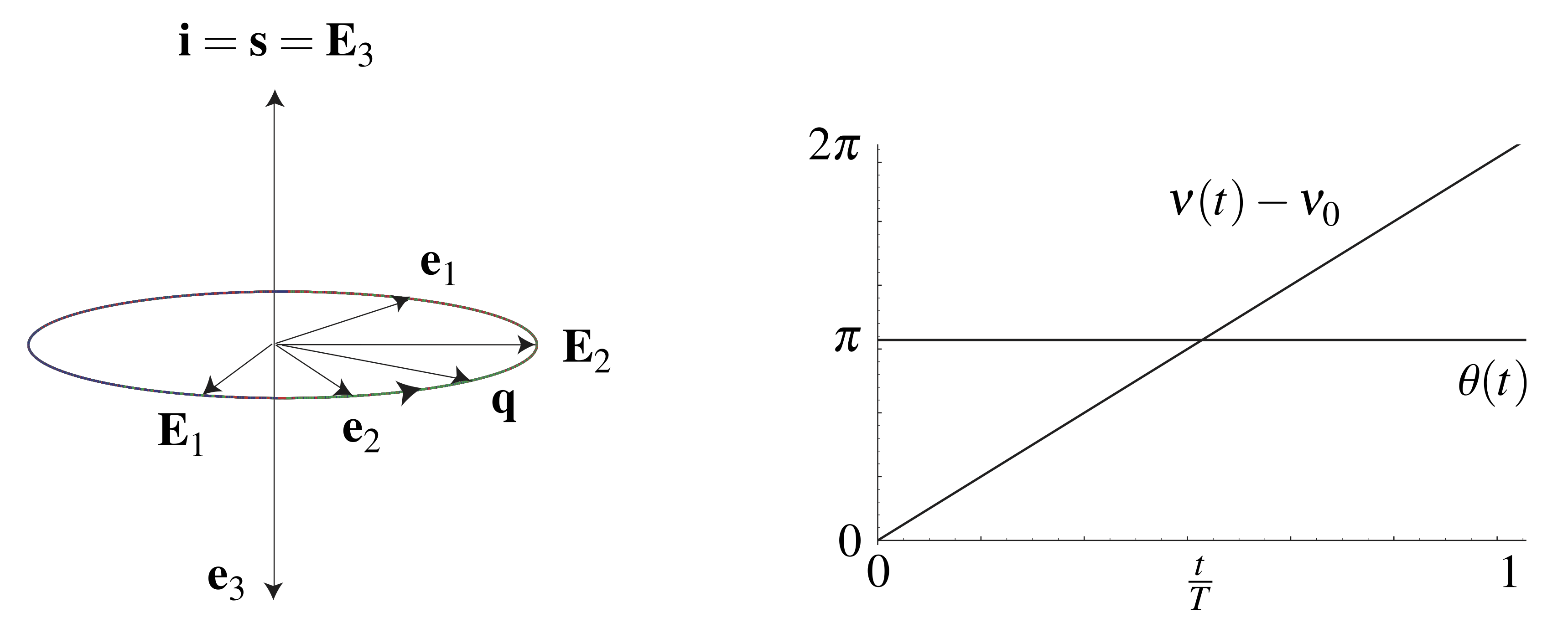

 and the rotation axes ,
  , and
, and  for the rotation tensor (27). Also shown in this figure is a plot of the angle
  that parameterizes the rotation axis and the angle of rotation
  about ; the parameter
  in this plot.
Notes
- Notice that if we choose the reference configuration and the initial state to be the same, then
 , and representations (7) and (9) are identical.
 - There are many ways to see this result. The simplest is to observe that the screw axis is in the null space of the tensor .
- We refer the interested reader to [7] and [8] for further discussion on this matter.
- This example is adapted from [9]. Other examples of rotations with constant angular velocity vectors but distinct rotation axes and can also be found in [9].
References
- Euler, L., Du mouvement de rotation des corps solides autour d’un axe variable, Mémoires de l’Académie des Sciences der Berlin 14 154–193 (1758). The title translates to “On the rotational motion of a solid body about a variable axis.” Reprinted in pp. 200–235 of Euler, L., Leonhardi Euleri Opera Omnia, II, Vol. 8, Orell Füssli, Zürich (1965). Edited by C. Blanc.
- Euler, L., Du mouvement d’un corps solides quelconque lorsqu’il tourne autour d’un axe mobile, Mémoires de l’Académie des Sciences der Berlin 16 176–227 (1760). The title translates to “On the motion of a solid body while it rotates about a moving axis.” Reprinted in pp. 313–356 of Euler, L., Leonhardi Euleri Opera Omnia, II, Vol. 8, Orell Füssli, Zürich (1965). Edited by C. Blanc.
- Whittaker, E. T., A Treatise on the Analytical Dynamics of Particles and Rigid Bodies, 4th ed., Cambridge University Press, Cambridge (1937).
- Casey, J., A treatment of rigid body dynamics, ASME Journal of Applied Mechanics 50(4a) 905–907 and 51 227 (1983).
- Poinsot, L., Outlines of a New Theory of Rotatory Motion, Translated from the French of Poinsot with Explanatory Notes, Cambridge University Press, London (1834). Translated from the French article “Théorie nouvelle de la rotation des corps présentée á l’Institut le 19 Mai 1834” by C. Whitley.
- Poisson, S. D., A Treatise of Mechanics, Longmans, London (1842). Translated from the French by H. H. Harte.
- Woltring, H. J., 3-D attitude representation of human joints: A standardization proposal, Journal of Biomechanics 27(12) 1399–1414 (1994).
- Woltring, H. J., Huiskes, R., de Lange, A., and Veldpaus, F. E., Finite centroid and helical axis estimation from noisy landmark measurements in the study of human joint kinematics, Journal of Biomechanics 18(5) 379–389 (1985).
- O’Reilly, O. M., and Payen, S., The attitudes of constant angular velocity motions, International Journal of Non-Linear Mechanics 41(7) 1–10 (2006).