There are two main problems in tracking and navigation. The first involves using data from targets rigidly attached to a body to determine the orientation and location of the body relative to a reference attitude and location. In many applications, the targets are optical and the data are recorded with a computer vision system. For example, in a variety of biomechanics applications, sets of optical targets are placed on two anatomical segments and the relative displacements of the targets are then used to measure the relative rotation  and translation
  of the two segments. It has long been known that the measurement of the rotation is difficult and prone to error. Several studies in the biomechanics community have discussed and quantified these errors for a variety of situations (e.g., see [1, 2, 3]). We devote this page to discussing various methods used to estimate and from sets of experimental data. These estimates are denoted by an asterisk, i.e.,
  and
and  . This problem is sometimes known as the Wahba problem [4] or the Procrustes problem [5].
Contents
Measurements and a cost function
Suppose we have a series of  current position measurement vectors
  associated with vectors of reference position measurements,
  . As shown in Figure 1, the reference and current measurements typically pertain to a set of targets, or landmarks, that are rigidly attached to the bodies of interest, and the motion of these objects is detected by cameras. The targets often come in fours so that they can be used to form a triad of vectors.
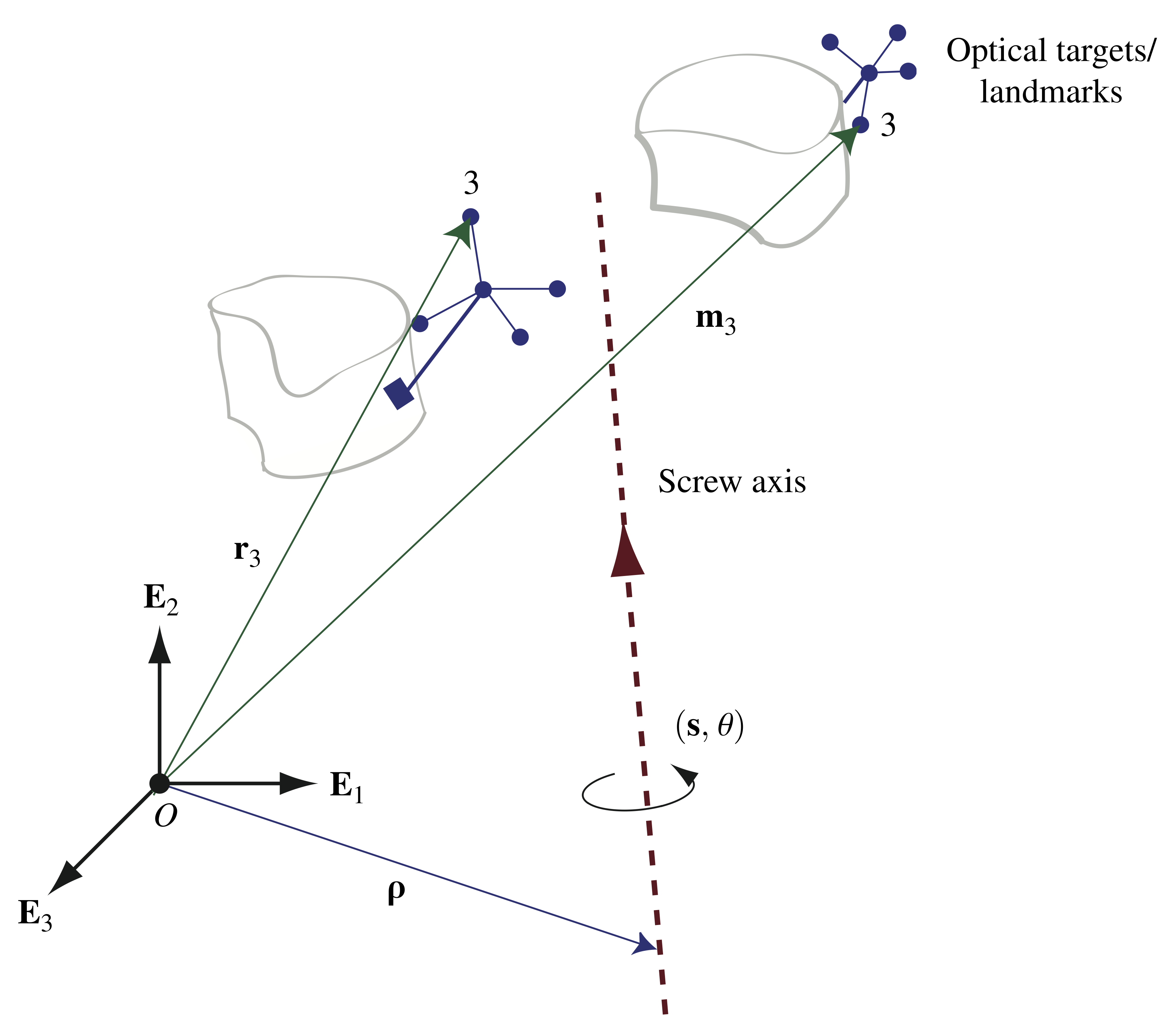
 , the screw axis, the rotation axis
  , and the angle of rotation,
  , are also shown.
Typically, the position measurements are all taken with respect to the same frame, which is often known as the laboratory frame:
(1) 
We wish to determine the rotation tensor  and translation
  that solves the equations
(2) 
Because of measurement errors, no unique solution  to these equations exist. The best we can do is to find the solution that minimizes the cost function
(3) 
where  are weights assigned to the individual measurements. Because
  is a rotation tensor, and thus proper-orthogonal, the cost function (3) is subject to the constraints
(4) 
An alternative decomposition of the motion given by (2) expresses this transformation in terms of the parameters of a helical (or screw) motion. As denoted in Figure 1, the four parameters for this motion are the rotation axis  that is parallel to the screw axis; the angle of rotation,
  , about this axis; the position vector of a point on the screw axis,
  ; and the translation
  along this axis. It is straightforward to show that and can be determined by solving the equation
(5) 
However, the tensor  is not invertible, so the solution for is not uniquely defined and indeed can be indeterminate when
  . One possibility is to choose to be the position vector from the origin to the screw axis that is normal to . Then, from (5), we find that
(6) ![\begin{eqnarray*} && {\brho} = \frac{1}{2}\left( {\bf d}_\perp + \cot\left( \frac{\theta}{2}\right) {\bf s}\times{\bf d} \right), \\ \\[0.10in] && \tau = {\bf s}\cdot{\bf d}, \end{eqnarray*}](https://rotations.berkeley.edu/wp-content/ql-cache/quicklatex.com-950f97d0a8baf3bbfc2ecd484d5e729a_l3.png "Rendered by QuickLaTeX.com")
where
(7) 
This solution to the parameters of the screw motion is equivalent to the one chosen by Spoor and Veldpaus in [6].
Solution methods
We now discuss four well-known solutions to the problem of estimating the rotation tensor and translation. We start with a naive approach that assumes there is no noise, measurement error, or finite precision issues. Next, a method from the satellite dynamics community known as the TRIAD method is discussed [7]. We then present a popular algorithm that uses the singular value decomposition of a matrix [8, 9]. We close with a discussion of the  -method, which employs unit quaternions (i.e., Euler-Rodrigues symmetric parameters) and features a novel eigenvalue problem [10, 11]. Comparisons of the methods we present can be found in works by Eggert et al. [12] and Metzger et al. [13]. We do not discuss error estimates for any of these methods. Instead, we refer the interested reader to Dorst’s paper [14]; his work enables one to correlate errors in the estimates and to noise and target distributions. Additional works in this area with specific application to biomechanics include studies by Panjabi [1], Spoor and Veldpaus [6], and Woltring et al. [2], among others.
A naive method
A naive method is to ignore errors in the measurement data and assume that one has four targets. First, we define the following augmented arrays for each target’s reference and current position measurement vectors:
(8) ![\begin{eqnarray*} && {\sf r}^{\prime}_K = \left[ \begin{array}{c} 1 \\ {\bf r}_K \cdot{\bf E}_1 \\ {\bf r}_K \cdot{\bf E}_2 \\ {\bf r}_K \cdot{\bf E}_3 \end{array} \right], \\ \\ \\ && {\sf m}^{\prime}_K = \left[\begin{array}{c} 1 \\ {\bf m}_K \cdot{\bf E}_1 \\ {\bf m}_K \cdot{\bf E}_2 \\ {\bf m}_K \cdot{\bf E}_3 \end{array} \right]. \end{eqnarray*}](https://rotations.berkeley.edu/wp-content/ql-cache/quicklatex.com-9506f272b72b8c78275de5e62e307d60_l3.png "Rendered by QuickLaTeX.com")
Assuming no errors in either the rotation or translation estimates, one can rewrite each of the four motion equations given by (2) in matrix-vector form as
(9) ![\begin{equation*} {\sf m}^{\prime}_K = \left[ \begin{array}{cc} 1 & {\sf 0} \\ {\sf d} & {\sf R} \end{array} \right]{\sf r}^{\prime}_K, \end{equation*}](https://rotations.berkeley.edu/wp-content/ql-cache/quicklatex.com-4d693deb716e3deaf5b64a900cb327f2_l3.png "Rendered by QuickLaTeX.com")
where
(10) ![\begin{eqnarray*} && {\sf R} = \left[ \begin{array}{c c c} R_{11} & R_{12} & R_{13} \\ R_{21} & R_{22} & R_{23} \\ R_{31} & R_{32} & R_{33} \end{array} \right] , \\ \\ \\ && {\sf d} = \left[ \begin{array}{c} {\bf d}\cdot{\bf E}_1 \\ {\bf d}\cdot{\bf E}_2 \\ {\bf d}\cdot{\bf E}_3 \end{array} \right]. \end{eqnarray*}](https://rotations.berkeley.edu/wp-content/ql-cache/quicklatex.com-953ec593d3e9b599a04c8379ee5b2c70_l3.png "Rendered by QuickLaTeX.com")
Given four non-coplanar targets, (9) can be used to solve for and :
(11) ![\begin{equation*} \left[\begin{array}{cc} 1 & {\sf 0} \\ {\sf d}^{*} & {\sf R}^{*} \end{array} \right] = \left[\begin{array}{cccc} {\sf m}^{\prime}_1 & {\sf m}^{\prime}_2 & {\sf m}^{\prime}_3 & {\sf m}^{\prime}_4 \end{array} \right] \left[\begin{array}{cccc} {\sf r}^{\prime}_1 & {\sf r}^{\prime}_2 & {\sf r}^{\prime}_3 & {\sf r}^{\prime}_4 \end{array} \right]^{-1}. \end{equation*}](https://rotations.berkeley.edu/wp-content/ql-cache/quicklatex.com-49d3006ab5e6353999d468a38e2f2286_l3.png "Rendered by QuickLaTeX.com")
Because there will always be some amount of noise and measurement error, the matrix  in (11) will typically not be proper-orthogonal. This fact contributes substantially to the errors observed when using this naive method.
The TRIAD method
The TRIAD algorithm is credited to Shuster and Oh [7] and dates to the early 1980s. It is often used with magnetometer, gravity, and star-pointing data, but here we consider the case where it is used with data obtained from optical targets. Given three sets of reference and current target position data, say,  and
and  , we can use these sets of vectors to define the right-handed orthonormal bases
  and
and  , respectively:
(12) 
and
(13) 
These unit vectors can be used to define two proper-orthogonal matrices:
(14) ![\begin{eqnarray*} && \mathsf{V} = \left[\begin{array}{c c c} {\bf V}_1\cdot{\bf E}_1 & {\bf V}_2\cdot{\bf E}_1 & {\bf V}_3\cdot{\bf E}_1\\ {\bf V}_1\cdot{\bf E}_2 & {\bf V}_2\cdot{\bf E}_2 & {\bf V}_3\cdot{\bf E}_2 \\ {\bf V}_1\cdot{\bf E}_3 & {\bf V}_2\cdot{\bf E}_3 & {\bf V}_3\cdot{\bf E}_3 \end{array} \right], \\ \\ \\ && \mathsf{v} = \left[\begin{array}{c c c} {\bf v}_1\cdot{\bf E}_1 & {\bf v}_2\cdot{\bf E}_1 & {\bf v}_3\cdot{\bf E}_1\\ {\bf v}_1\cdot{\bf E}_1 & {\bf v}_2\cdot{\bf E}_2 & {\bf v}_3\cdot{\bf E}_2 \\ {\bf v}_1\cdot{\bf E}_1 & {\bf v}_2\cdot{\bf E}_3 & {\bf v}_3\cdot{\bf E}_3 \end{array} \right]. \end{eqnarray*}](https://rotations.berkeley.edu/wp-content/ql-cache/quicklatex.com-9ba3fad26668ffb5f58456804c11c4d5_l3.png "Rendered by QuickLaTeX.com")
With the help of the motion equations (2), we can manipulate  and
and  to solve for the matrix
  :
:
(15) 
The translation vector  is then calculated using the mean positions of the targets before and after the motion:
(16) 
where
(17) 
For a set of four targets, there are 24 possible constructions of the matrices  and
and  , and thus 24 possible estimates of and . To obtain the optimal and , we examine the error
  between the true and calculated positions of the targets after the motion:
(18) ![\begin{equation*} {e}^2=\lnorm \left[{\bf m}_1, \, {\bf m}_2, \, {\bf m}_3, \, {\bf m}_4 \right]-\left({\bf R}\left[{\bf r}_1, \, {\bf r}_2, \, {\bf r}_3, \, {\bf r}_4 \right] + \left[{\bf d}, \, {\bf d}, \, {\bf d}, \, {\bf d} \right]\right) \rnorm. \end{equation*}](https://rotations.berkeley.edu/wp-content/ql-cache/quicklatex.com-a205f118692b73775da0a45987551635_l3.png "Rendered by QuickLaTeX.com")
The rotation tensor and translation that yield the smallest error are considered the optimal results  .
.
A method based on the singular value decomposition
The method featuring the singular value decomposition (SVD) is credited to Arun et al. [8] and to Hanson and Norris [9] in the 1980s. Additional discussions of this method can be found in [15, 16, 17]. The first step of the SVD method involves computing the mean positions for a set of four targets before and after the motion:
(19) 
Next, a matrix is formed using position vectors relative to these mean positions:
(20) 
where
(21) ![\begin{eqnarray*} && {\sf C} = \left[\begin{array}{c c c c} \left({\bf m}_1 - \overline{\bf m}\right)\cdot{\bf E}_1 & \left({\bf m}_2 - \overline{\bf m}\right)\cdot{\bf E}_1 & \left({\bf m}_3 - \overline{\bf m}\right)\cdot{\bf E}_1 & \left({\bf m}_4 - \overline{\bf m}\right) \cdot{\bf E}_1 \\ \left({\bf m}_1 - \overline{\bf m}\right)\cdot{\bf E}_2 & \left({\bf m}_2 - \overline{\bf m}\right)\cdot{\bf E}_2 & \left({\bf m}_3 - \overline{\bf m}\right)\cdot{\bf E}_2 & \left({\bf m}_4 - \overline{\bf m}\right) \cdot{\bf E}_2 \\ \left({\bf m}_1 - \overline{\bf m}\right)\cdot{\bf E}_3 & \left({\bf m}_2 - \overline{\bf m}\right)\cdot{\bf E}_3 & \left({\bf m}_3 - \overline{\bf m}\right)\cdot{\bf E}_3 & \left({\bf m}_4 - \overline{\bf m}\right) \cdot{\bf E}_3 \end{array} \right], \hspace{1in} \scalebox{0.001}{\textrm{\textcolor{white}{.}}} \\ \\ \\ && {\sf D} = \left[\begin{array}{c c c c} \left({\bf r}_1 - \overline{\bf r}\right)\cdot{\bf E}_1 & \left({\bf r}_2 - \overline{\bf r}\right)\cdot{\bf E}_1 & \left({\bf r}_3 - \overline{\bf r}\right)\cdot{\bf E}_1 & \left({\bf r}_4 - \overline{\bf r}\right) \cdot{\bf E}_1 \\ \left({\bf r}_1 - \overline{\bf r}\right)\cdot{\bf E}_2 & \left({\bf r}_2 - \overline{\bf r}\right)\cdot{\bf E}_2 & \left({\bf r}_3 - \overline{\bf r}\right)\cdot{\bf E}_2 & \left({\bf r}_4 - \overline{\bf r}\right) \cdot{\bf E}_2 \\ \left({\bf r}_1 - \overline{\bf r}\right)\cdot{\bf E}_3 & \left({\bf r}_2 - \overline{\bf r}\right)\cdot{\bf E}_3 & \left({\bf r}_3 - \overline{\bf r}\right)\cdot{\bf E}_3 & \left({\bf r}_4 - \overline{\bf r}\right) \cdot{\bf E}_3 \end{array} \right]. \end{eqnarray*}](https://rotations.berkeley.edu/wp-content/ql-cache/quicklatex.com-c00ccd39218c36d57fbb2c7730b2266d_l3.png "Rendered by QuickLaTeX.com")
We then calculate the singular value decomposition of  :
:
(22) 
where  and
and  are orthogonal matrices, and
  is a 3
  3 diagonal matrix. Finally, the optimal estimates of the rotation and translation are given by
(23) ![\begin{eqnarray*} && {\sf R}^{*} = {\sf R}_1 \left[ \begin{array}{c c c} 1 & 0 & 0 \\ 0 & 1 & 0 \\ 0 & 0 & \mbox{det}\left({\sf R}_1{\sf R}_2\right) \end{array} \right] {\sf R}_2, \\ \\[0.15in] && {\bf d}^{*} = \overline{\bf m} - {\bf R}^{*}{\overline{\bf r}}. \end{eqnarray*}](https://rotations.berkeley.edu/wp-content/ql-cache/quicklatex.com-9090d8d78042e197655414dbad633628_l3.png "Rendered by QuickLaTeX.com")
The q-method
The -method dates to the latter half of the 20th century. The method uses unit quaternions (i.e., Euler-Rodrigues symmetric parameters) to parameterize the rotation and features a novel eigenvalue problem to arrive at an estimate for the optimal rotation. This solution was developed independently by Davenport [10] and later in a well-cited paper by Horn [11]. To show how the  -method works, we start by defining the parameter
  and the “centers” of the reference and current position measurements based on assigned weights :
(24) 
Expanding the cost function given in (3), we find with some straightforward manipulations that
(25) 
We are interested in extremizing  as a function of the rotation tensor and translation , so we can ignore the underbraced terms in (25) that are independent of and . In short, we wish to find and that maximize
(26) 
We now parameterize using a set of Euler-Rodrigues symmetric parameters,  :
:
(27) ![\begin{equation*} \mathsf{R} = \left(e^2_0 - e^2_1 - e^2_2 - e^2_3\right) \left[ \begin{array}{c c c} 1 & 0 & 0 \\ 0 & 1 & 0 \\ 0 & 0 & 1 \\ \end{array} \right] + \left[ \begin{array}{c c c} 2e^2_1 & 2e_1e_2 & 2e_1e_3 \\ 2e_1e_2 & 2e^2_2 & 2e_2e_3 \\ 2e_1e_3 & 2e_2e_3 & 2e^2_3 \\ \end{array} \right] + \left[ \begin{array}{c c c} 0 & - 2 e_0 e_3 & 2 e_0 e_2 \\ 2 e_0 e_3 & 0 & - 2 e_0 e_1 \\ - 2 e_0 e_2 & 2 e_0 e_1 & 0 \\ \end{array} \right]. \hspace{1in} \scalebox{0.001}{\textrm{\textcolor{white}{.}}} \end{equation*}](https://rotations.berkeley.edu/wp-content/ql-cache/quicklatex.com-04245c651436ae1c178b3144d43c3cf1_l3.png "Rendered by QuickLaTeX.com")
This representation enables us to express (26) in a more compact form:
(28) 
where the 4 4 symmetric matrix  and the column vector are given by
(29) ![\begin{eqnarray*} && \mathsf{K} = \left[ \begin{array}{c c} \mathsf{B} + \mathsf{B}^T - \mbox{tr}\left(\mathsf{B}\right) \mathsf{I} & \mathsf{z} \\ \mathsf{z}^T & \mbox{tr}\left(\mathsf{B}\right) \end{array} \right], \\ \\ \\ && \mathsf{q} = \left[ \begin{array}{c} e_1 \\ e_2 \\ e_3 \\ e_0 \end{array} \right]. \end{eqnarray*}](https://rotations.berkeley.edu/wp-content/ql-cache/quicklatex.com-1439b7c3cb97b1b7c1f428e5fbdf31c2_l3.png "Rendered by QuickLaTeX.com")
Here,  is the 3 3 identity matrix, the column vector
(30) ![\begin{equation*} \renewcommand\arraystretch{1.5} \mathsf{z} = \left[\begin{array}{c} \left( {\bf m}\times{\bf r} - \frac{1}{\alpha} \sum_{K \, \, = \, 1}^N \alpha_K {\bf m}_K\times{\bf r}_K\right)\cdot{\bf E}_1 \\ \left( {\bf m}\times{\bf r} - \frac{1}{\alpha} \sum_{K \, \, = \, 1}^N \alpha_K {\bf m}_K\times{\bf r}_K\right)\cdot{\bf E}_2 \\ \left( {\bf m}\times{\bf r} - \frac{1}{\alpha} \sum_{K \, \, = \, 1}^N \alpha_K {\bf m}_K\times{\bf r}_K \right)\cdot{\bf E}_3 \end{array} \right], \end{equation*}](https://rotations.berkeley.edu/wp-content/ql-cache/quicklatex.com-170f0f582636a661fd335708dcc3d89e_l3.png "Rendered by QuickLaTeX.com")
and the 3 3 matrix ![\mathsf{B} = \left [ B_{ij} \right ]](https://rotations.berkeley.edu/wp-content/ql-cache/quicklatex.com-a27c7cb085c325c216b48207fb7aa2e6_l3.png "Rendered by QuickLaTeX.com")
 , for which the components
(31) 
Note that the matrices  and are composed entirely of measurements. Our definition of the column vector
  differs by a minus sign from that found in the literature for the case when
  (e.g., see [7, 18]). This difference is expected and can be traced to our convention for the skew-symmetric part of the matrix in (27).
We are now in a position to solve for the optimal and . Specifically, we seek and that maximize (28), subject to the Euler parameter constraint  . With the help of a Lagrange multiplier
  , one seeks
  and that maximize
(32) 
It is now straightforward to calculate the optimal solution by differentiating  with respect to its arguments. Doing so, one finds
(33) 
That is, the optimal is an eigenvector of . For to be maximized,  must be the eigenvector corresponding to the largest eigenvalue of . Once this eigenvector is found, can be constructed using (27). Notice that
  is a simple mean value, but it can only be obtained after
  has been determined. You should also notice that because the 4 4 matrix is real and symmetric, it has four real eigenvalues and its eigenvectors are orthogonal. One advantage of the -method is that determining the rotation axis
  and the corresponding rotation angle
  for the screw axis representation of the motion follows easily once is known:
(34) 
An example of estimating a rigid-body motion
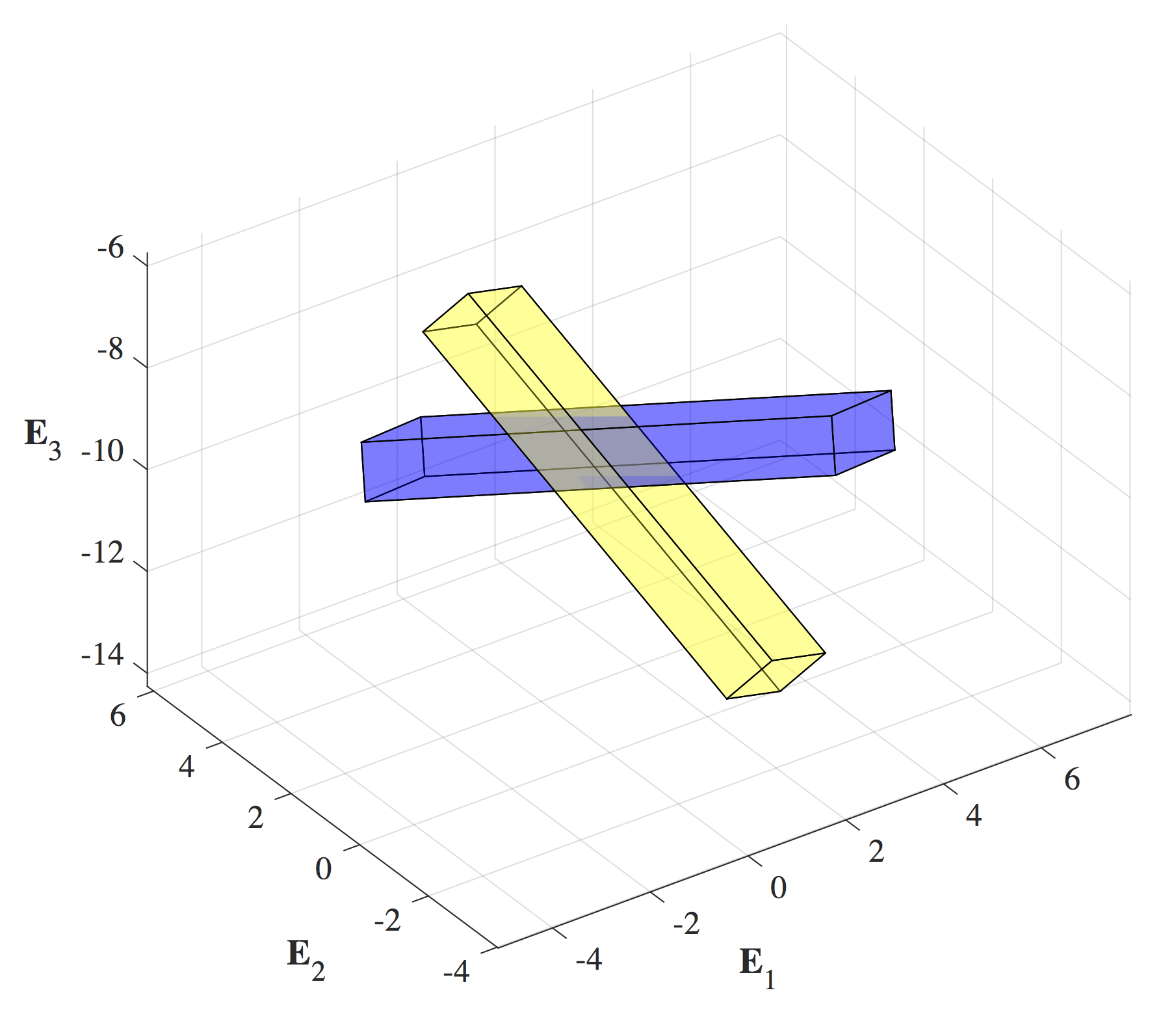
To illustrate the four methods for estimating rotations and translations from measurement data, we consider the example of a tossed book. Referring to Figure 2, we choose four landmark points on a uniform rectangular prism of length  , width
  , and thickness
  such that their position vectors in the reference state are
(35) 
For the example at hand, we choose the dimensions  ,
,  , and
, and  (with units of inches) to mimic a small book. Note that in the reference state, the body’s center of mass
  is located at the origin and the rotation tensor can be taken as the identity transformation, i.e., in the reference configuration.

 and current configuration
  of a tossed book represented by a uniform rectangular prism, with the landmark points used for calculations labeled 1 through 4.
Suppose we rotate and translate the book such that at time  , the book’s orientation and translation are described by, respectively,
(36) ![\begin{eqnarray*} && {\bf R} = {\bf L}\left( \phi = \frac{\pi}{4}, \, {\bf e}_1\right){\bf L}\left( \theta = \frac{\pi}{6}, \, {\bf e}^{\prime}_2\right){\bf L}\left( \psi = \frac{\pi}{4}, \, {\bf E}_3\right), \hspace{1in} \scalebox{0.001}{\textrm{\textcolor{white}{.}}} \\ \\[0.15in] && {\bf d} = {\bf E}_1 + {\bf E}_2 - 10{\bf E}_3, \end{eqnarray*}](https://rotations.berkeley.edu/wp-content/ql-cache/quicklatex.com-8c7abc02a60739eb9a294f61aad0108a_l3.png "Rendered by QuickLaTeX.com")
where, using a 3-2-1 set of Euler angles to parameterize , the rotation axis  . A lengthy but straightforward calculation shows that the components of at time are
(37) ![\begin{equation*} \mathsf{R} = \left[ \begin{array}{c c c} R_{11} & R_{12} & R_{13} \\ R_{21} & R_{22} & R_{23} \\ R_{31} & R_{32} & R_{33} \\ \end{array} \right] = \left[ \begin{array}{c c c} \sqrt{\frac{3}{8}} & - \frac{1}{4} & \frac{3}{4} \\ \sqrt{\frac{3}{8}} & \frac{3}{4} & - \frac{1}{4} \\ - \frac{1}{2} & \sqrt{\frac{3}{8}} & \sqrt{\frac{3}{8}} \\ \end{array} \right]. \end{equation*}](https://rotations.berkeley.edu/wp-content/ql-cache/quicklatex.com-d62e54e194c8dd7213b65105e3817a78_l3.png "Rendered by QuickLaTeX.com")
In terms of Euler’s representation, the rotation  is equivalent to a counterclockwise rotation of
  about an axis
(38) 
We assume there is no noise in the measurements, in which case, using (2), the landmark points’ position vectors at time are
(39) 
We now examine how the four methods described earlier estimate and at time using the position measurements (35) and (39). The forthcoming results that we present were calculated in MATLAB; the associated code is available for download here.
Solution using the naive method
The solution procedure for the naive method reveals that the augmented matrix in (11) is
(40) ![\begin{equation*} \left[ \begin{array}{c c} 1 & \mathsf{0} \\ \mathsf{d}^* & \mathsf{R}^* \end{array} \right] = \left[ \begin{array}{c c c c} 1 & 0 & 0 & 0 \\ 1.0000 & 0.6124 & -0.2500 & 0.7500 \\ 1.0000 & 0.6124 & 0.7500 & -0.2500 \\ -10.0000 & -0.5000 & 0.6124 & 0.6124 \end{array} \right], \hspace{1in} \scalebox{0.001}{\textrm{\textcolor{white}{.}}} \end{equation*}](https://rotations.berkeley.edu/wp-content/ql-cache/quicklatex.com-cab479530602dcef4dc4e3323c00851e_l3.png "Rendered by QuickLaTeX.com")
and so
(41) ![\begin{eqnarray*} && {\mathsf R}^* = \left[ \begin{array}{c c c} 0.6124 & -0.2500 & 0.7500 \\ 0.6124 & 0.7500 & -0.2500 \\ -0.5000 & 0.6124 & 0.6124 \end{array} \right], \\ \\ \\ && {\mathsf d}^* = \left[ \begin{array}{c} 1.0000 \\ 1.0000 \\ -10.0000 \end{array} \right]. \end{eqnarray*}](https://rotations.berkeley.edu/wp-content/ql-cache/quicklatex.com-129df50f8e7032db9486b37042e2a4c8_l3.png "Rendered by QuickLaTeX.com")
Within numerical precision, the resulting predictions of and are accurate.
Solution using the TRIAD method
Out of 24 possible permutations, the matrix  that has the least error, as defined by (18), is given by
(42) ![\begin{equation*} \mathsf{R}^* = \mathsf{v}\mathsf{V}^{T} = \left[\begin{array}{c c c} -0.2500 & -0.7500 & -0.6124 \\ 0.7500 & 0.2500 & -0.6124 \\ 0.6124 & -0.6124 & 0.5000 \end{array} \right] \left[ \begin{array}{c c c} 0 & 0 & -1 \\ 1 & 0 & 0 \\ 0 & -1 & 0 \end{array} \right]^{T}. \hspace{1in} \scalebox{0.001}{\textrm{\textcolor{white}{.}}} \end{equation*}](https://rotations.berkeley.edu/wp-content/ql-cache/quicklatex.com-6629827227fd8f9cb4a338abb85d8920_l3.png "Rendered by QuickLaTeX.com")
The resulting  is identical to that estimated by the naive method; the same is true of the translation.
Solution using the method based on the singular value decomposition
The matrix  in (20) is calculated as
(43) ![\begin{equation*} {\mathsf S} = {\mathsf C}{\mathsf D}^T = \left[ \begin{array}{c c c c} -1.7872 & 3.1117 & -0.2872 & -1.0372 \\ -0.0372 & 4.8617 & -4.5372 & -0.2872 \\ 1.7655 & -2.2345 & -1.9088 & 2.3778 \end{array} \right] \left[ \begin{array}{c c c c} -2 & 6 & -2 & -2 \\ 1.5 & 1.5 & -4.5 & 1.5 \\ -0.25 & -0.25 & -0.25 & 0.75 \end{array} \right]^T. \hspace{1in} \scalebox{0.001}{\textrm{\textcolor{white}{.}}} \end{equation*}](https://rotations.berkeley.edu/wp-content/ql-cache/quicklatex.com-61adec3fe9d6fcb212202747af8ece43_l3.png "Rendered by QuickLaTeX.com")
To compute the singular value decomposition of in MATLAB, we use the built-in singular value decomposition function ![\texttt{[U,X,V] = svd(S)}](https://rotations.berkeley.edu/wp-content/ql-cache/quicklatex.com-e9df6042403b17e88955b11d8863a0c4_l3.png "Rendered by QuickLaTeX.com") , where
, where  ,
,  , and
, and  . In this case,
(44) ![\begin{eqnarray*} && {\mathsf R}_1 = \left[ \begin{array}{c c c} -0.4378 & 0.3987 & 0.8058 \\ -0.8724 & -0.4052 & -0.2735 \\ 0.2174 & -0.8227 & 0.5253 \end{array} \right], \\ \\ \\ && {\mathsf R}_2^T = \left[ \begin{array}{c c c} -0.9110 & 0.4074 & 0.0633 \\ -0.4117 & -0.9074 & -0.0849 \\ 0.0228 & -0.1035 & 0.9944 \end{array} \right]. \end{eqnarray*}](https://rotations.berkeley.edu/wp-content/ql-cache/quicklatex.com-6f7d95de199fe49040177264515d28de_l3.png "Rendered by QuickLaTeX.com")
Both and have unit determinant, and so, from (23)1,
(45) 
which agrees with the estimates from the naive and TRIAD methods. A subsequent calculation involving (23)2 shows that the translation estimate also agrees with the two earlier methods.
Solution using the q-method
Using (29), (30), and (31) with unit weights 
 , the matrices
  and
and  are given by
(46) ![\begin{eqnarray*} && \mathsf{B} = \left[ \begin{array}{c c c} 6.2235 & 0.4309 & -0.2593 \\ 9.7235 & 6.8059 & -0.0718 \\ -4.4691 & 2.8632 & 0.5945 \end{array} \right], \\ \\ \\ && \mathsf{K} = \left[ \begin{array}{c c c c} -1.1769 & 10.1543 & -4.7284 & 2.9350 \\ 10.1543 & -0.0121 & 2.7913 & 4.2098 \\ -4.7284 & 2.7913 & -12.4349 & 9.2926 \\ 2.9350 & 4.2098 & 9.2926 & 13.6238 \end{array} \right]. \end{eqnarray*}](https://rotations.berkeley.edu/wp-content/ql-cache/quicklatex.com-70fb7dd6c6a5d9132bfc51e6bd4b4448_l3.png "Rendered by QuickLaTeX.com")
The eigenvalues of are all real. The eigenvector that corresponds to the largest eigenvalue is
(47) ![\begin{equation*} {\mathsf q}^* = \left[ \begin{array}{c} 0.2500 \\ 0.3624 \\ 0.2500 \\ 0.8624 \end{array} \right]. \end{equation*}](https://rotations.berkeley.edu/wp-content/ql-cache/quicklatex.com-f76e053e5f806ead3f539156945bfe51_l3.png "Rendered by QuickLaTeX.com")
When we construct  from the components of
  using (27), we find that the estimate of the rotation is the same as those computed by the naive, TRIAD, and singular value decomposition methods; the same is true of the translation when we calculate it from (33)2 after obtaining . This equivalence can be attributed to the noiseless nature of the measurements. Lastly, when the rotation has the representation
  , it can be shown from using (34) that the angle and axis of rotation are, respectively,
(48) 
which agree with their expected values from earlier.
The effect of measurement noise
In the absence of noise, it is well known that the four methods give equally accurate results, and this was observed in the previous calculations. However, in the presence of noise, this situation changes. To illustrate this point, we numerically added noise to the landmark points’ current position measurements 
 and recomputed the rotation and translation estimates. We found that the naive and TRIAD methods were susceptible to noise, while the SVD method and the -method were equally accurate. Figure 3 depicts the difference between the book’s actual orientation and location at time and its configuration estimated by the TRIAD method when are subject to noise.

 .
.Downloads
The MATLAB files used to perform calculations and generate Figure 3 for the example we discussed in this page are available here and here. The former file is the main script that executes the calculations and plots the actual and estimated configurations; the latter is a function called by the main script to draw the book in these plots.
References
- Panjabi, M. M., Centers and angles of rotation of body joints: A study of errors and optimization, Journal of Biomechanics 12(12) 911-920 (1979).
- Woltring, H. J., Huiskes, R., de Lange, A., and Veldpaus, F. E., Finite centroid and helical axis estimation from noisy landmark measurements in the study of human joint kinematics, Journal of Biomechanics 18(5) 379–389 (1985).
- Yuan, X., Ryd, L., and Blankevoort, L., Error propagation for relative motion determined from marker positions, Journal of Biomechanics 30(9) 989-992 (1997).
- Wahba, G., Problem 65-1, A least squares estimate of satellite attitude, SIAM Review 8(3) 384–386 (1966).
- Schönemann, P. H., A generalized solution of the orthogonal Procrustes problem, Psychometrika 31(1) 1–10 (1966).
- Spoor, C. W., and Veldpaus, F. E., Rigid body motion calculated from spatial co-ordinates of markers, Journal of Biomechanics 13(4) 391-393 (1980).
- Shuster, M. D., and Oh, S. D., Three-axis attitude determination from vector observations, Journal of Guidance, Control, and Dynamics 4(1) 70–77 (1981).
- Arun, K. S., Huang, T. S., and Blostein, S. D., Least-squares fitting of two 3-D point sets, IEEE Transactions on Pattern Analysis and Machine Intelligence 9(5) 698-700 (1987).
- Hanson, R. J., and Norris, M. J., Analysis of measurements based on the singular value decomposition, SIAM Journal on Scientific and Statistical Computing 2(3) 363-373 (1981).
- Keat, J., Analysis of Least-Squares Attitude Determination Routine DOAOP, CSC Report CSC/TM-77/6034 (February 1977).
- Horn, B. K. P., Closed-form solution of absolute orientation using unit quaternions, Journal of the Optical Society of America A 4(4) 629–642 (1987).
- Eggert, D. W., Lorusso, A., and Fisher, R. B., Estimating 3-D rigid body transformations: A comparison of four major algorithms, Machine Vision and Applications 9(5–6) 272–290 (1997).
- Metzger, M. F., Faruk Senan, N. A., O’Reilly, O. M., and Lotz, J. C., Minimizing errors associated with calculating the helical axis for spinal motions, Journal of Biomechanics 43(14) 2822-2829 (2010).
- Dorst, L., First order error propagation of the Procrustes method for 3D attitude estimation, IEEE Transactions on Pattern Analysis & Machine Intelligence 27(2) 221–229 (2005).
- Markley, F. L., Attitude determination using vector observations and the singular value decomposition, Journal of the Astronautical Sciences 36(3) 245–258 (1988).
- Markley, F. L., Attitude determination using vector observations: A fast optimal matrix algorithm, Journal of the Astronautical Sciences 41(2) 261-280 (1993).
- Söderkvist, I., and Wedin, P. A., Determining the movements of the skeleton using well-configured markers, Journal of Biomechanics 26(12) 1473–1477 (1993).
- Bar-Itzhack, I. Y., REQUEST: A recursive QUEST algorithm for sequential attitude determination, Journal of Guidance, Control, and Dynamics 19(5) 1034-1038 (1996).